|
IMC '05 Paper
[IMC '05 Technical Program]


Joint Data Streaming and Sampling Techniques for Detection of Super Sources and Destinations
Qi (George) Zhao Abhishek Kumar Jun (Jim) Xu
College of Computing, Georgia Institute of Technology
Abstract:
Detecting the sources or destinations that have communicated with a
large number of distinct destinations or sources
during a small time interval
is an important problem in network measurement and security.
Previous detection approaches
are not able to deliver the desired accuracy
at high link speeds (10 to 40 Gbps). In
this work, we propose two novel algorithms that provide
accurate and efficient solutions to this problem. Their designs are
based on the insight that sampling and data streaming are often suitable
for capturing different and complementary regions of the information
spectrum, and a close collaboration between them is an excellent way to
recover the complete information. Our first solution builds on the
standard hash-based flow sampling algorithm.
Its main innovation is that the sampled traffic
is further filtered by a data streaming module
which allows for much higher sampling rate and hence much
higher accuracy.
Our second
solution is more sophisticated but offers higher accuracy. It
combines the power of data streaming in efficiently
estimating
quantities
associated with a given identity, and the power of sampling in
collecting a list of candidate identities. The performance of both
solutions are evaluated using both mathematical analysis and
trace-driven experiments on real-world Internet traffic.
1 Introduction
Measurement of flow-level statistics, such as total active flow count,
sizes and identities of large flows, per-flow traffic, and flow size
distribution are essential for network management and
security. Measuring such information on high-speed links (e.g., 10
Gbps) is challenging since the standard method of maintaining per-flow
state (e.g., using a hash table) for tracking various flow statistics
is prohibitively expensive. More specifically, at very high link
speeds, updates to the per-flow state for each and every incoming
packet would be feasible only through the use of very fast and
expensive memory (typically SRAM), while the size of such state is
very large [7] and hence too expensive to be held in SRAM.
Recently, the techniques for approximately measuring such statistics using
a much smaller state, based on a general methodology called
network data streaming, have been used to solve some of the
aforementioned problems
[5,6,12,11,22]. The main idea in
network data streaming is to use a small and fast memory to process
each and every incoming packet in real-time. Since it is impractical
to store all information in this small memory, the principle of data
streaming is to maintain only the information most pertinent to the
statistic to be measured.
In this work, we design data streaming algorithms that help detect super
sources and destinations.
A super source![[*]](footnote.png) is
a source that has a large fan-out (e.g., larger than a
predefined threshold) defined as the number of distinct destinations
it communicates with during a small time interval.
The concepts of super destination and fan-in can be defined
symmetrically. Our schemes in fact solve a strictly harder problem
than making a binary decision of whether a source/destination is a
super source/destination or not: They actually provide accurate
estimates of the fan-outs/fan-ins of potential super
sources/destinations.
In this work a source can be any combination of ``source'' fields
from a packet header such as source IP address, source port
number, or their combination, depending on target applications.
Similarly, a destination can be any combination of the
``destination'' fields from a packet header. We refer to the
source-destination pair of a packet as the flow label and use
these two terms interchangeably in the rest of this paper. is
a source that has a large fan-out (e.g., larger than a
predefined threshold) defined as the number of distinct destinations
it communicates with during a small time interval.
The concepts of super destination and fan-in can be defined
symmetrically. Our schemes in fact solve a strictly harder problem
than making a binary decision of whether a source/destination is a
super source/destination or not: They actually provide accurate
estimates of the fan-outs/fan-ins of potential super
sources/destinations.
In this work a source can be any combination of ``source'' fields
from a packet header such as source IP address, source port
number, or their combination, depending on target applications.
Similarly, a destination can be any combination of the
``destination'' fields from a packet header. We refer to the
source-destination pair of a packet as the flow label and use
these two terms interchangeably in the rest of this paper.
The problem of detecting super sources and destinations arises in many
applications of network monitoring and security. For example,
port-scans probe for the existence of vulnerable services
across the Internet by trying to connect to many different pairs of
destination IP address and port number. This is clearly a type of super source under our definition.
Similarly, in a DDoS (Distributed Denial of Service) attack, a large
number of zombie hosts flood packets to a destination. Thus the
problem of detecting the launch of DDoS attacks can be viewed as
detecting a super destination. This problem also arises in detecting
worm propagation and estimating their spreading rates. An infected host
often propagates the worm to a large number of destinations, and can
be viewed as a super source. Knowing its fan-out allows us to
estimate the rate at which the worm may spread. Another possible
instance lies in peer-to-peer and content distribution networks, where
a few servers or peers might attract a larger number of requests (for
content) than they can handle while most of others in the network are
relatively idle. Being able to detect such ``hot spots'' (a type of
super destination) in real-time helps balance the workload and improve
the overall performance of the network. A number of other variations
of the above applications, such as detecting flash crowds
[9] and reflector attacks [15], also motivate
this problem.
Techniques proposed in the literature for solving this problem
typically maintain per-flow state, and cannot scale to high link
speeds of 10 or 40 Gbps. For example, to detect port-scans, the
widely deployed Intrusion Detection System (IDS) Snort
[19] maintains a hash table of the distinct
source-destination pairs to count the destinations each source talks
to. A similar technique is used in FlowScan [17] for
detecting DDoS attacks.
The inefficiency in such an approach stems from the fact that most of
the source-destination pairs are not a part of port scans or DDoS
attacks. Yet, they result in a large number of source-destination
pairs that can be accommodated only in DRAM, which cannot support the
high access rates required for updates at line speed.
More recent work [20] has offered solutions based on
hash-based flow sampling technique. However, its accuracy is limited
due to the typically low sampling rate imposed by some inherent
limitations of the hash-based flow sampling technique discussed later
in Section 3. A more comprehensive survey of related
work is provided in Section 7.
In this paper we propose two efficient and accurate data streaming
algorithms for detecting the set of super sources by estimating the
fan-outs of the collected sources.
These algorithms can be easily adapted symmetrically for detecting the
super destinations. Their designs are based on the insight that
(flow) sampling and data streaming are often suitable for capturing
different and complementary regions of the information spectrum, and a
close collaboration between them is an excellent way to recover the
complete information. This insight leads to two novel methodologies
of combing the power of streaming and sampling, namely, ``filtering
after sampling'' and ``separation of counting and identity
gathering''. Our two solutions are built upon these two methodologies
respectively.
Our first solution, referred to as the simple scheme, is based
on the methodology of ``filtering after sampling''. It enhances the
traditional hash-based flow sampling algorithm to approximately count
the fan-outs of the sampled sources. As suggested by its name, the
design of this solution is very simple. Its main innovation is that
the sampled traffic is further filtered by a simple data streaming
module (a bit array), which guarantees that at most one packet from
each flow is processed. This allows for much higher sampling rate
(hence much higher accuracy) than achievable with traditional
hash-based flow sampling. Our second solution, referred to as the
advanced scheme, is more sophisticated than the simple scheme
but offers even higher accuracy. Its design is based on the
methodology of ``separation of counting and identity gathering'',
which combines the power of streaming in efficiently estimating
quantities (e.g., fan-out) associated with a given identity, and the
power of sampling in generating a list of candidate identities (e.g.,
sources). Through rigorous theoretical analysis and extensive
trace-driven experiments on real-world Internet traffic, we
demonstrate these two algorithms produce very accurate fan-out
estimations.
We also extend our advanced scheme for detecting the sources that have
large outstanding fan-outs, defined as the number of distinct
destinations it has contacted but has not obtained acknowledgments
(TCP ACK) from.
This extension has several important applications. One example is that
in port-scans, the probing packets, which target a large number of
destinations, will receive acknowledgments from only a small
percentage of them. Another example is distributed TCP SYN attacks.
In this case, the victim's TCP acknowledgments (SYN/ACK packets) to a
large number of hosts for completing the TCP handshake (the second
step) are not acknowledged. Our evaluation on bidirectional traffic
collected simultaneously on a link shows that our solution estimates
outstanding fanout with high accuracy.
The rest of this paper is organized as follows. In the next section,
we present our design methodologies and provide an overview of the
proposed solutions. Sections 3 and 4
describe the design of the two schemes in detail respectively and
provide a theoretical analysis of their complexity and
accuracy. Section 5 presents an extension of our scheme
for estimating outstanding fan-outs. We evaluate our solutions in
Section 6 using packet header traces of real-world
Internet traffic. We discuss the related work in Section 7
before concluding in Section 8.
2 Overview of our schemes
As we mentioned above, accurate measurement and monitoring in high
speed networks are challenging because the traditional per-flow schemes
cannot scale to high link speeds. As a stop-gap solution, packet
sampling has been used to keep up with high link speeds. In packet
sampling, a small fraction  of traffic is sampled and
processed. Since the sampled packets constitute a much lower volume
than the original traffic, a per-flow table stored in relatively
inexpensive DRAM can handle all the updates triggered by the sampled
packets in real-time [14]. Thus we can typically obtain
complete information contained in the sampled traffic. The statistics
of the original traffic are then inferred from that of the sampled
traffic by ``inverting'' the sampling process, i.e., by compensating
for the effects of sampling. However the accuracy of such
sampling-based estimations is usually low, because the error is scaled
by of traffic is sampled and
processed. Since the sampled packets constitute a much lower volume
than the original traffic, a per-flow table stored in relatively
inexpensive DRAM can handle all the updates triggered by the sampled
packets in real-time [14]. Thus we can typically obtain
complete information contained in the sampled traffic. The statistics
of the original traffic are then inferred from that of the sampled
traffic by ``inverting'' the sampling process, i.e., by compensating
for the effects of sampling. However the accuracy of such
sampling-based estimations is usually low, because the error is scaled
by  and is typically small (e.g., 1/500) to make the sampling
operation computationally
affordable [4,11,8]. In other words, although
the sampling-based approach allows for 100% accurate digesting of
information on sampled traffic, a large amount of information may be
lost during the sampling process. and is typically small (e.g., 1/500) to make the sampling
operation computationally
affordable [4,11,8]. In other words, although
the sampling-based approach allows for 100% accurate digesting of
information on sampled traffic, a large amount of information may be
lost during the sampling process.
Network data streaming has begun to be recognized as a better alternative to
sampling for measurement and monitoring of high-speed
links [10].
Contrary to sampling, a network data streaming algorithm will process
each and every packet passing through a high-speed link to glean
the most important information for answering a specific type of query,
using a small yet well-organized data structure. This data structure
is small enough to be fit into fast (yet expensive) SRAM, allowing it
to keep up with high link speeds. The challenge is to design this
data structure in such a way that it encodes the information we need,
for answering the query, in a succinct manner. Data streaming
algorithms, if available, typically offer much more accurate
estimations than sampling for measuring network flow statistics. This
is because, intuitively the sampling throws away a large percentage of
information up front, while data streaming, which processes each and
every packet, is often able to retain most of the most important
information inside a small SRAM module.
In our context of detecting super sources, however, both sampling and
data streaming are valuable for capturing different and complementary
regions of the information spectrum, and a close collaboration between
them is used to recover the complete information.
There are two parts of information that we would like to
know in finding super sources: one is the identities (e.g., IP
addresses) of the sources that may be super sources. The other is the
fan-out associated with each source identity.
We observe that data
streaming algorithms can encode the fan-outs of various
sources into a very succinct data structure. Such a data structure,
however, typically only provides a lookup interface. In other words,
if we obtain a source identity through other means, we are able to
look up the data structure to obtain its (approximate) fan-out, but
the data structure itself cannot produce any
identities and is undecodable without such identities being supplied
externally. On the other hand, sampling is an excellent way of
gathering source identities though it is not a great counting device
as we described earlier.
The above observation leads to one of the two aforementioned design
methodologies, i.e., separating identity gathering and counting.
The idea is to use a streaming data structure as a counting device and
use sampling
to gather the identities of potential super sources. Then we look up
the streaming data structure using the gathered identities to obtain the
corresponding counts. This methodology is used in our advanced scheme
that employs a 2-dimensional bit array as the counting device, in
parallel with an identity gathering module that adopts an enhanced
form of sampling. We show that our
sampling module has vanishingly small probability of missing the
identity of any actual super sources and the estimation
module produces highly accurate estimates of the fan-out of the potential
super sources. This scheme is especially suitable for very
high link speeds of 10 Gbps and above. We describe this scheme in
Section 4.
We also explore another way of combing sampling and streaming,
i.e., ``filtering after sampling''. Its idea is to employ a data
streaming module between the sampling operation and the final processing
procedure to efficiently encode whether a flow has been seen
before.
A careful design of this module guarantees that at most one packet in
each flow needs to be processed. This allows us to achieve
much higher sampling rate and hence much higher accuracy than the
traditional flow sampling scheme.
This solution works very well for relatively lower link speeds
(e.g., 10 Gbps and below).
We describe this scheme in detail in Section 3.
3 The simple scheme
In this section we present a relatively simple scheme for detecting
super sources. It builds upon the traditional hash-based flow sampling
technique but can achieve a much higher sampling rate, and hence more
accurate estimation. We begin with a discussion of some limitations of
the traditional hash-based sampling approach, and then describe our
solution that alleviates these limitations. We also present an
analysis of the complexity and accuracy of the scheme.
1 Limitations of traditional hash-based flow sampling
There are two generic sampling approaches for network measurement:
packet sampling and flow sampling. In the former approach, each packet
is sampled independently with a certain probability, while in the
latter, the sampling decision is made at the granularity of flows
(i.e., all packets belonging to sampled flows are sampled). In the
following, we only consider flow sampling since packet sampling is not
suitable for our context of detecting super sources.
A traditional flow sampling algorithm that estimates the fan-outs of
sources works
as follows. The algorithm randomly samples a certain percentage (say
) of source-destination pairs using a hashing technique (described
next). The fan-out of each source in the sampled pairs is counted and
then scaled by to obtain an estimate of the fan-out of the
source in the original traffic (i.e., before sampling). This counting
process is typically performed using a hash table that
stores the fan-out values (after sampling) of all sources seen
in the sampled traffic so far, and a newly sampled flow will
increment the fan-out counter of the corresponding hash node (or
trigger the creation of a new node). Since the estimation error is
also scaled by , it is desirable to make the sampling rate as
high as possible. However, we will show that, at high link speeds,
the traditional hash-based flow sampling approach may prevent us from
achieving high sampling rate needed for accurate estimation.
Flow sampling is commonly implemented using a simple hashing technique
[3] as follows. First a hash function  that maps
a flow label to a value uniformly distributed in that maps
a flow label to a value uniformly distributed in  is fixed.
When a packet arrives, its flow label is hashed by . Given a
sampling probability , the flow is sampled if and only if the
hashing result is no more than . Recall that the purpose of flow
sampling is to reduce the amount of traffic that needs to be processed
by the aforementioned hash table which performs the counting.
Clearly, it is desirable that a hash table that runs slightly faster
than times the link speed, can keep up with the incoming rate of
the sampled traffic (with rate ). For example, we would like a
hash table (in DRAM) that is able to process a packet in is fixed.
When a packet arrives, its flow label is hashed by . Given a
sampling probability , the flow is sampled if and only if the
hashing result is no more than . Recall that the purpose of flow
sampling is to reduce the amount of traffic that needs to be processed
by the aforementioned hash table which performs the counting.
Clearly, it is desirable that a hash table that runs slightly faster
than times the link speed, can keep up with the incoming rate of
the sampled traffic (with rate ). For example, we would like a
hash table (in DRAM) that is able to process a packet in  to
handle all traffic sampled from a link with 10 million packets per
second (i.e., one packet arrival per to
handle all traffic sampled from a link with 10 million packets per
second (i.e., one packet arrival per  on the average) with
slightly less than 25% sampling rate. Unfortunately, we cannot
achieve this goal with the current hash-based flow sampling approach
for the following reason. on the average) with
slightly less than 25% sampling rate. Unfortunately, we cannot
achieve this goal with the current hash-based flow sampling approach
for the following reason.
With hash-based flow sampling, if a flow is
sampled, all packets belonging to the flow need to be processed by the
hash table. Internet traffic is very bursty in the sense that the
packets belonging to a flow tend to arrive in bursts and do not
interleave well with packets from other flows and is also known to
exhibit the following characteristic [5]: a small
number of elephant flows contain most of the overall traffic while the
vast majority of the flows are small. If a few elephant flows are
sampled, their packets could generate a long burst of sampled traffic
that has much higher rate than that can be handled by the hash
table. Therefore,
with hash-based flow sampling, the sampling rate has to be much
smaller than the ratio between the operating speed of the hash table
and the arrival rate of traffic, thus leading to large estimation
errors as discussed before.
In the following subsection, we present an efficient yet simple
solution to this problem, allowing the sampling rate to reach or even
well exceed this ratio.
In [20] the authors propose a
one-level filtering algorithm which uses the
hash-based flow sampling approach described above, in conjunction
with a hash table for counting the fan-out values. It does
not specify whether DRAM or SRAM will be used to implement the hash
table. If DRAM were used, it will not be able to achieve a high
sampling rate as discussed before. If SRAM were used, the memory
cost is expected to be prohibitive when the sampling rate is high.
This algorithm appears to be effective and
accurate for monitoring lower link speeds, but cannot deliver a high
estimation accuracy when operating at high link speeds such as 10Gbps (the
target link speeds are not mentioned in
[20]).
Figure 1:
Traditional flow sampling vs. filtering after sampling
|
2 Our scheme
We design a filtering technique that completely
solves the aforementioned problem. It allows the sampling rate to be
very close to the ratio between the hash table speed and the link
speed in the worst-case and well exceed the ratio otherwise.
Its conceptual design is shown
in Figure 1. Compared with the traditional flow
sampling approach, our approach places a data streaming module between
the hash-based flow sampling module and the hash table (for counting).
This streaming module guarantees that at most one packet from each
sampled flow needs to be processed by the hash table. This will
completely smooth out the aforementioned traffic bursts in the
flow-sampled traffic, since such bursts are caused by highly bursty
arrivals from one or a small number of elephant flows and now only the
first packets of these flows may trigger updates to the hash table.
Figure 2:
Algorithm of updating data streaming module.
|
|
The data structure and algorithm of the data streaming module are shown
in Figure 2. Its basic idea is to use a bit
array  to remember whether a flow label,
a source-destination pair in our context, has been
processed by the hash table.
Let the size of the array be to remember whether a flow label,
a source-destination pair in our context, has been
processed by the hash table.
Let the size of the array be  bits. We fix a hash function bits. We fix a hash function  that maps
a flow label to a value uniformly distributed in that maps
a flow label to a value uniformly distributed in ![$ [1, w]$](img24.png) .
The array is initialized to all ``0''s at the beginning of a measurement epoch.
Upon the arrival of a packet .
The array is initialized to all ``0''s at the beginning of a measurement epoch.
Upon the arrival of a packet  , we hash its flow label ( , we hash its flow label (
 ) using and the result ) using and the result  is treated
as an index into the array . If is treated
as an index into the array . If ![$ G[r]$](img28.png) is equal to 1, our algorithm
concludes that a packet with this flow label has been processed
earlier, and takes no further action. Otherwise (i.e., is 0), this
flow label will be processed to update the corresponding counter is equal to 1, our algorithm
concludes that a packet with this flow label has been processed
earlier, and takes no further action. Otherwise (i.e., is 0), this
flow label will be processed to update the corresponding counter
 maintained in a hash table maintained in a hash table  .
Then is set to 1 to remember the fact that a packet with this
flow has been seen and processed. This method clearly ensures that at
most one packet from each sampled flow is processed by . However,
due to hash collisions, some sampled flows may not be processed at all
since their corresponding bits in would be set by their colliding
counterparts. The update procedure of the hash table
, described next, statistically compensates for such collisions. .
Then is set to 1 to remember the fact that a packet with this
flow has been seen and processed. This method clearly ensures that at
most one packet from each sampled flow is processed by . However,
due to hash collisions, some sampled flows may not be processed at all
since their corresponding bits in would be set by their colliding
counterparts. The update procedure of the hash table
, described next, statistically compensates for such collisions.
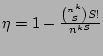
Now we explain our statistical estimator, which is the computation
result of the hash table update procedure shown in
Figure 2 (line 11). Suppose the number of ``0''
entries in (with size ) is  right before a packet with
source right before a packet with
source  arrives ( arrives (
 in line 10). Assume belongs
to a new flow and its flow label hashes to an index . The value of
has value 0 with probability in line 10). Assume belongs
to a new flow and its flow label hashes to an index . The value of
has value 0 with probability
 . Therefore to obtain an
unbiased estimator . Therefore to obtain an
unbiased estimator
 of the fan-out of the source on
the sampled traffic, we should statistically compensate for the fact
that with probability of the fan-out of the source on
the sampled traffic, we should statistically compensate for the fact
that with probability
 , the bit has value 1 and
will miss the update to due to aforementioned hash
collisions. It is intuitive that if we add , the bit has value 1 and
will miss the update to due to aforementioned hash
collisions. It is intuitive that if we add
 to
, the resulting estimator is unbiased. To be more
precise, suppose in a measurement epoch, the hash table is updated by
altogether to
, the resulting estimator is unbiased. To be more
precise, suppose in a measurement epoch, the hash table is updated by
altogether  packets { packets { , ,
 } from a source ,
whose flow labels hash to locations } from a source ,
whose flow labels hash to locations  's where 's where
![$ G[r_j] = 0$](img42.png) , and
there are , and
there are  0's in right before arrives, respectively.
The output of the hash table , which is an unbiased estimator of
the fan-out of on the sampled traffic, is 0's in right before arrives, respectively.
The output of the hash table , which is an unbiased estimator of
the fan-out of on the sampled traffic, is
 |
(1) |
We show in the following lemma that this is an unbiased estimator of  and its proof can be found in [24].
Lemma 1
is an unbiased estimator of , i.e.,
![$ E[\widehat{N_s}]=N_s$](img46.png) . .
Then an unbiased estimator of the fan-out  of source is
given by scaling
by , i.e., of source is
given by scaling
by , i.e.,
where is the sampling rate used in the flow sampling. We
show in the following theorem that the estimator
 is
unbiased. Its proof uses Lemma 1 and is also provided in
[24]. is
unbiased. Its proof uses Lemma 1 and is also provided in
[24].
Theorem 1
is an unbiased estimator of , i.e.,
![$ E[\widehat{F_s}]=F_s$](img49.png) . .
We now demonstrate that this solution will completely smooth out the
aforementioned problem of traffic bursts
, and allow the sampling rate
to be close to the ratio between the hash table speed and the link
rate, the theoretical upper limit in the worst case. The worst case
for our scheme is that each flow contains only one packet (e.g., in
the case of DDoS attacks). Even in this
worst case, the update times to the hash table (viewed as a random
process) is very close to Poisson (nonhomogeneous as the value of varies over
time) since each new flow is sampled independently. Due to the
``benign'' nature of this arrival process, by employing a tiny SRAM
buffer (e.g., holding 20 flow labels of 64  100 bits each), a hash
table that operates slightly faster than the average rate of this
process will only miss a negligible fraction of updates due to buffer
overflow. This process can be faithfully modeled as a Markov chain for
rigorous analysis. We elaborate it with a numerical example in
[24] and omit it here due to lack of space. 100 bits each), a hash
table that operates slightly faster than the average rate of this
process will only miss a negligible fraction of updates due to buffer
overflow. This process can be faithfully modeled as a Markov chain for
rigorous analysis. We elaborate it with a numerical example in
[24] and omit it here due to lack of space.
Notice that in Figure 2 the variable , the number
of ``0'' entries in , decreases as more and more sampled flows are
processed. When more and more packets pass through the data streaming
module, becomes small and hence the probability for a new flow to be
recorded,
, decreases. Thereby the estimation error
will increase.
To maintain high accuracy, we specify a minimum value  for
. Once the value of drops below , the estimation
procedure will use a new array (set to all ``0''s initially) and start
a new measurement epoch (with an empty hash table). Two sets of
arrays and hash tables will be operated in an alternating manner so
that the measurement can be performed without interruption. The
parameter is typically set to around for
. Once the value of drops below , the estimation
procedure will use a new array (set to all ``0''s initially) and start
a new measurement epoch (with an empty hash table). Two sets of
arrays and hash tables will be operated in an alternating manner so
that the measurement can be performed without interruption. The
parameter is typically set to around  (i.e., ``half full''). (i.e., ``half full'').
3 Complexity analysis
The above scheme has extremely low storage (SRAM) complexity and
allows for very high streaming speed.
Memory (SRAM) consumption. Each processed flow
only consumes a little more than one bit in SRAM.
Thus a reasonable amount of SRAM can support very high link speeds.
For example, assuming the average flow size of 10 packets [11],
512KB SRAM is enough to support a measurement epoch which
is slightly longer than 2 seconds for a link with 10 million packets
per second even without performing any flow sampling. With 25% flow
sampling which is typically set for OC-192 links the SRAM requirement is
even brought down to 128KB.
Streaming speed. Our algorithm in
Figure 2 has two branches to deal with the packets
arriving at the data streaming module. If the corresponding bit is ``1'',
the packets only require one hash function computation and one read to
SRAM. Otherwise they require one hash function computation, one read
and one write (at the same location) to SRAM and an update to the hash
table. Using efficient hardware implementation of hash function
[18] and  SRAM, all operations in the data streaming
module can be finished in 10's of SRAM, all operations in the data streaming
module can be finished in 10's of  in both cases. in both cases.
4 Accuracy analysis
Now we establish the following theorem to characterize the variance of
the estimator
in Formula 2. Its proof can be
found in [24]
Remark: The above variance consists of two terms. The
first term corresponds to the variance of the error term in estimating
the sampled fan-out, scaled by
 (to compensate for
sampling), and the second term corresponds to the variance of the
error term in inverting flow sampling process. Since these two errors
are approximately orthogonal to each other, their total variance is
the sum of their individual variances. (to compensate for
sampling), and the second term corresponds to the variance of the
error term in inverting flow sampling process. Since these two errors
are approximately orthogonal to each other, their total variance is
the sum of their individual variances.
4 The advanced scheme
In this section we propose the advanced scheme that is more sophisticated
than the simple scheme but can offer more accurate fan-out
estimations. It is based on
the aforementioned design methodology of separating identity gathering from
counting.
Its system model is shown in
Figure 3. There are two parallel modules processing
the incoming packet stream. The data streaming module encodes the
fan-out information for each and every source (arc 1 in
Figure 3) into a very compact data structure, and the
identity sampling module captures the candidate source identities which have
potential to be super sources (arc 2). These source identities are
then used by an estimation algorithm to look up the data
structure (arc 3) produced by the data streaming module (arc 4) to get their
corresponding fan-out
estimates. The design of these modules are described in the following
subsections.
Figure 3:
System model of the advanced scheme
|
Figure 4:
An instance of online streaming module
|
Figure 5:
Algorithm of online streaming module
|
|
The data structure used in the online streaming module is quite simple:
an
 2-dimensional bit array 2-dimensional bit array  . The bits in are set
to all ``0''s at the beginning of each measurement epoch. The
algorithm of updating is shown in
Figure 5. Upon the arrival of a packet , . The bits in are set
to all ``0''s at the beginning of each measurement epoch. The
algorithm of updating is shown in
Figure 5. Upon the arrival of a packet ,
 is hashed by is hashed by  independent hash functions independent hash functions
 with range with range ![$ [1..n]$](img67.png) . The hashing results . The hashing results
 , ,
 , ..., , ...,
 are viewed as
column indices into . In our scheme, is set to 3, and the
rationale behind it will be discussed in Section 4.3. Then,
the flow label
is hashed by another independent
hash function are viewed as
column indices into . In our scheme, is set to 3, and the
rationale behind it will be discussed in Section 4.3. Then,
the flow label
is hashed by another independent
hash function  (with range (with range ![$ [1..m]$](img72.png) ) to generate a row index of
. Finally, the bits located at the intersections of the
selected row and columns are set to ``1''. An example is shown in
Figure 4, in which the three intersection bits (circled)
are set to ``1''s. When is filled (by ``1'') to a threshold
percentage we terminate the current measurement epoch and start the
decoding process.
In Section 4.2, we show that the above process
produces a very compact and accurate (statistical) encoding of the
fan-outs of the sources, and present the corresponding decoding
algorithm. ) to generate a row index of
. Finally, the bits located at the intersections of the
selected row and columns are set to ``1''. An example is shown in
Figure 4, in which the three intersection bits (circled)
are set to ``1''s. When is filled (by ``1'') to a threshold
percentage we terminate the current measurement epoch and start the
decoding process.
In Section 4.2, we show that the above process
produces a very compact and accurate (statistical) encoding of the
fan-outs of the sources, and present the corresponding decoding
algorithm.
Readers may feel that the above 2D bit array is a variant of
Bloom filters [1]. This is not the case since although its
encoding algorithm is similar to that of a Bloom filter (flipping some
bits to ``1"s), we decode the 2D bit array for a different kind of
information (the fan-out count) than if we really use it as a Bloom
filter (check if a particular source-destination pair has
appeared). Our encoding algorithm is not well engineered for being used
as a Bloom filter. And our decoding algorithm, shown next, is also
fundamentally different from that of a Bloom filter.
The proposed online streaming module has very low memory consumption
and high streaming speed:
Memory (SRAM) consumption. Our scheme is extremely
memory-efficient. Each source-destination pair (flow) will set 3 bits
in the bit vectors to ``1''s and consume a little more than 3 bits of SRAM
storage. We will show that
the scheme provides very high accuracy using reasonable amount of
SRAM (e.g., 128KB) in Section 6.
Streaming speed. Each update requires only  hash
function computations and hash
function computations and  writes to the SRAM.
We require that these four hash functions
are independent and amendable to hardware implementation.
They can be chosen from the writes to the SRAM.
We require that these four hash functions
are independent and amendable to hardware implementation.
They can be chosen from the  hash function family [2,18],
which, with hardware implementation, can produce a hash output within
a few nanoseconds. Then with commodity
SRAM our scheme would allow around hash function family [2,18],
which, with hardware implementation, can produce a hash output within
a few nanoseconds. Then with commodity
SRAM our scheme would allow around  million packets per second,
thereby supporting Gbps traffic stream assuming a conservative
average packet size of 1,000 bits. million packets per second,
thereby supporting Gbps traffic stream assuming a conservative
average packet size of 1,000 bits.
2 Estimation module
For each source identity recorded by the sampling module (described
later), the estimation module decodes its approximate fan-out from the
2D bit array , the output of the data streaming module.
In this section, we describe this decoding algorithm in detail.
When we would like to know , the fan-out of the source ,
is hashed by the hash functions  , ,  , ,  , which are
defined and used in the online streaming module, to obtain column
indices. Let , which are
defined and used in the online streaming module, to obtain column
indices. Let  , ,  , 2, , , be the corresponding
columns (viewed as bit vectors). In the following, we derive, step by
step, an accurate and almost unbiased estimator of , as a
function of , , 2, , . , 2, , , be the corresponding
columns (viewed as bit vectors). In the following, we derive, step by
step, an accurate and almost unbiased estimator of , as a
function of , , 2, , .
Let the set of packets hashed into column during the
corresponding measurement epoch be  and the number of bits in
that are ``0''s be and the number of bits in
that are ``0''s be  . Note that the value is a
part of our observation since we can obtain from
through simple counting, although the notation itself contains ,
the size of which we would like to estimate. Recall the size of the
column vector is . Note that the value is a
part of our observation since we can obtain from
through simple counting, although the notation itself contains ,
the size of which we would like to estimate. Recall the size of the
column vector is  . A fairly accurate estimator of . A fairly accurate estimator of  , the
number of packets of , adapted from [21], is , the
number of packets of , adapted from [21], is
Note that , the fan-out of the source , is equal to
 , if during the measurement epoch, no other
sources are hashed to the same columns , if during the measurement epoch, no other
sources are hashed to the same columns
 .
Otherwise
is the sum of the
fan-outs of all (more than 1) the sources that are hashed into
. We show in the next section, that the
probability with which the latter case happens is very small when .
Otherwise
is the sum of the
fan-outs of all (more than 1) the sources that are hashed into
. We show in the next section, that the
probability with which the latter case happens is very small when  .
We obtain the following estimator of , which is in fact derived
as an estimator for
. .
We obtain the following estimator of , which is in fact derived
as an estimator for
.
Here
 , is defined as , is defined as
 , where , where
 denotes the number of ``0''s in the bit vector denotes the number of ``0''s in the bit vector
 which is the result of hashing the set of packets which is the result of hashing the set of packets
 into a single empty bit vector. The bit
vector
is computed as the bitwise-OR of
,..., into a single empty bit vector. The bit
vector
is computed as the bitwise-OR of
,...,  . One can easily verify the correctness of this
computation with respect to the semantics of
. . One can easily verify the correctness of this
computation with respect to the semantics of
.
We need to show that the RHS of Formula 4 is a fairly
good estimator of
. Note that
by the principle of inclusion and exclusion. Since
is a fairly good estimator of
 according to [21], we obtain the RHS of
Formula 4 by replacing the terms
in Formula 5 by
, according to [21], we obtain the RHS of
Formula 4 by replacing the terms
in Formula 5 by
,
 . Note that it is not correct to directly use the
bitwise-AND of . Note that it is not correct to directly use the
bitwise-AND of
 for estimating
using Formula 3, because the bit vector
corresponding to the result of hashing the set of packets for estimating
using Formula 3, because the bit vector
corresponding to the result of hashing the set of packets
 into an empty bit vector, is not equivalent to
the bitwise-AND of into an empty bit vector, is not equivalent to
the bitwise-AND of
 . .
The estimator in Formula 4 generalizes the result
in [21] which is
developed for the special case  . We will show that our scheme only needs to use the special case of
, which is . We will show that our scheme only needs to use the special case of
, which is
The computational complexity of estimating the fan-out of a source is
dominated by  bitwise-OR operations among column vectors.
Such vectors can be encoded as one or more unsigned integers so that
the bit-parallelism can significantly reduce the execution time.
Since is typically 64 bits in our scheme, the whole vector can be
held in two 32-bit integers. Therefore, in our scheme where ,
estimation of the fan-out of each source only needs 8
bitwise-OR operations between 32-bit integers.
We also need to count the number of ``0''s in a vector (to get bitwise-OR operations among column vectors.
Such vectors can be encoded as one or more unsigned integers so that
the bit-parallelism can significantly reduce the execution time.
Since is typically 64 bits in our scheme, the whole vector can be
held in two 32-bit integers. Therefore, in our scheme where ,
estimation of the fan-out of each source only needs 8
bitwise-OR operations between 32-bit integers.
We also need to count the number of ``0''s in a vector (to get  values). This can be sped up significantly by using a pre-computed
table (in SRAM) of size 262,144 (
values). This can be sped up significantly by using a pre-computed
table (in SRAM) of size 262,144 (
 ) bits that stores
the number of ``0''s
in all 16-bit numbers. Our estimation of the execution time shows
that our scheme is fast enough to support OC-768 operations. ) bits that stores
the number of ``0''s
in all 16-bit numbers. Our estimation of the execution time shows
that our scheme is fast enough to support OC-768 operations.
3 Accuracy analysis
In this section we first briefly explain the rationale behind setting
to in the estimator and then analyze the accuracy of our estimator
rigorously.
We set (the number of ``column'' hash functions) to 3 due to the
following two considerations.
First, we mentioned before that if two sources  and and  both
are hashed to the same columns, our decoding algorithm will give
us an estimate of their total fan-out, when we use
or to lookup the 2D array. We certainly would like the
probability with which
this scenario occurs to be as small as possible. This can be achieved
by making as large as possible. However, larger implies
larger computational and storage complexities at the online streaming
module. We will show that makes the probability of the
aforementioned hash collision very small, and at the same time keeps
the computational and storage complexities of our scheme modest. both
are hashed to the same columns, our decoding algorithm will give
us an estimate of their total fan-out, when we use
or to lookup the 2D array. We certainly would like the
probability with which
this scenario occurs to be as small as possible. This can be achieved
by making as large as possible. However, larger implies
larger computational and storage complexities at the online streaming
module. We will show that makes the probability of the
aforementioned hash collision very small, and at the same time keeps
the computational and storage complexities of our scheme modest.
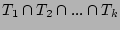
Now we derive  , the probability that at least two sources
happen to hash to the same set of columns by , , the probability that at least two sources
happen to hash to the same set of columns by ,
 , ..., . It is not hard to show, using straightforward
combinatorial arguments, that , ..., . It is not hard to show, using straightforward
combinatorial arguments, that
 , where , where  is the total number of the distinct sources
during the measurement epoch. We observe that, given typical values for is the total number of the distinct sources
during the measurement epoch. We observe that, given typical values for
 and , is quite large when , but drops to a very low
value when . For example, when and , is quite large when , but drops to a very low
value when . For example, when  K and K and  ,
is close to ,
is close to  when , but drops to when , but drops to  when . when .
The following theorem characterizes the variance of the estimator in
Formula 6, which is also its approximate mean square
error (MSE), since the estimator is almost unbiased and the impact of
(discussed above) on the estimation error is very small when
. Its proof can be found in [24]. This is an extension
of our previous variance analysis in [23] which is derived
for the special case .
Let  denote denote  , which is the load factor of the bit
vector(of size ) when the corresponding set , which is the load factor of the bit
vector(of size ) when the corresponding set  of
source-destination pairs are hashed into it, in the following theorem. of
source-destination pairs are hashed into it, in the following theorem.
Theorem 3
The variance of
is given by
where
 . .
Figure 6:
Distribution of the estimation from Monte-Carlo simulation ( b, and b, and  ). ).  is the standard deviation computed from Theorem 3 is the standard deviation computed from Theorem 3
|
An example distribution of
with respect to the actual
value is shown in Figure 6. We obtained this
distribution with 20,000 runs of the Monte-Carlo simulations with the
following parameters. In this empirical distribution, the actual
fan-out is 50, the size of the column vector is 64 bits.
The load factor is set to
 for for
 . Also,
since the sets . Also,
since the sets  , ,  , and , and  have 50 flows in common, we
set have 50 flows in common, we
set
 , for , for
 . Here we implicitly assume that pairs of them do not have any
flows in common other than these 50 flows, which happens with very
high probability ( . Here we implicitly assume that pairs of them do not have any
flows in common other than these 50 flows, which happens with very
high probability (
 ) anyway given a
large (e.g., 16K).
In this example the standard deviation is around ) anyway given a
large (e.g., 16K).
In this example the standard deviation is around  as
computed from Theorem 3. We observe that the size of
the tail that falls outside 2 standard deviations from the mean is
very small ( as
computed from Theorem 3. We observe that the size of
the tail that falls outside 2 standard deviations from the mean is
very small ( ). This shows that, with high probability, our
estimator will not deviate too much from the actual value. In
Section 6, the trace-driven experiments on the
real-world Internet traffic will further validate this. ). This shows that, with high probability, our
estimator will not deviate too much from the actual value. In
Section 6, the trace-driven experiments on the
real-world Internet traffic will further validate this.
Note that given the size of , our scheme is only able to accurately
estimate fan-out values up to
 , because if the actual
fan-out is much larger than that, we will see all 1's in the
corresponding column vectors with high probability (due to the result
of the ``coupon collector's problem'' [13]). In this
case, the only information we can obtain about is that it is no
smaller than , because if the actual
fan-out is much larger than that, we will see all 1's in the
corresponding column vectors with high probability (due to the result
of the ``coupon collector's problem'' [13]). In this
case, the only information we can obtain about is that it is no
smaller than  . Fortunately, for the purpose of detecting
super sources, this information is good enough for us to declare a
super source, as long as the threshold for super sources is much
smaller than . However, in some applications (e.g.,
estimating the spreading speed of a worm), we may also want to know
the approximate fan-out value. This can be achieved using a
multi-resolution extension of our advanced scheme. The methodology
of multi-resolution is quite standard and has been used in
several recent works [6,12,11]. The extension in
our context is straightforward. We omit its detailed specifications
here in interest of space. . Fortunately, for the purpose of detecting
super sources, this information is good enough for us to declare a
super source, as long as the threshold for super sources is much
smaller than . However, in some applications (e.g.,
estimating the spreading speed of a worm), we may also want to know
the approximate fan-out value. This can be achieved using a
multi-resolution extension of our advanced scheme. The methodology
of multi-resolution is quite standard and has been used in
several recent works [6,12,11]. The extension in
our context is straightforward. We omit its detailed specifications
here in interest of space.
4 Identity sampling module
The purpose of this module is to capture the identities of
potential super sources
that will be used to look up the 2D array to get their
fan-out estimations. The filtering after sampling technique
proposed in Section 3 is adopted here with a slightly
different recording strategy. Instead of constructing a hash table to
record the sources and their fan-out estimation, here we only record
the source identities sequentially in the DRAM. Since this strategy
avoids expensive hash table operations and sequential writes to DRAM
can be made very fast (using burst mode), very high sampling rate can
be achieved.
With commodity SRAM and  DRAM, this recording strategy
will be able to process more than 12.5 million packets per second. At
this speed, we can record 100% and 25% flow labels for OC-192 and
OC-768 links respectively. With such a high sampling rate, the
probability that the identity of a real super source misses sampling is
very low. For example, given 25% sampling rate the probability that
a source with fan-out 50 fails to be recorded is only DRAM, this recording strategy
will be able to process more than 12.5 million packets per second. At
this speed, we can record 100% and 25% flow labels for OC-192 and
OC-768 links respectively. With such a high sampling rate, the
probability that the identity of a real super source misses sampling is
very low. For example, given 25% sampling rate the probability that
a source with fan-out 50 fails to be recorded is only
 (= (=
 ). ).
5 Estimating outstanding fan-outs
In this section we describe how to extend the advanced scheme to
detect the sources that have contacted but have not obtained
acknowledgments from a large number of distinct destinations (i.e.,
the sources with large outstanding fan-outs).
Although both of our schemes have the potential to support this
extension we focus on the advanced scheme in this work and leave the
extension of the simple scheme for future research. In the following
sections we show how to slightly modify the operations of the online
streaming module and the estimation module of the advanced scheme for
estimating outstanding fan-outs. The sampling module does not need to
be modified.
Figure 7:
Algorithm for updating the 2D bit array  to record ACK packets to record ACK packets
|
|
The online streaming module employs two 2D bit arrays and
of identical size and shape.
The array encodes the fan-outs of sources in traffic in one
direction (called ``outbound'') in the same way as in the advanced
scheme (shown in Figure 5). The array encodes the
fan-ins of the destinations of the acknowledgment packets in the
opposite direction (called ``inbound'').
Its encoding algorithm is shown in Figure 7. It
is a transposed version of the algorithm shown in
Figure 5 in the sense that all occurrences of
``'' are replaced with with `` '' and ``''
with ``''. This transposition is needed since a source in
the outbound traffic appears in the inbound acknowledgment traffic as
a destination, and after transposing two packets that belong to a flow
and its ``acknowledgment flow'' respectively will result in a write of
``1'' to the same bit locations in and respectively. This
allows us to essentially take a ``difference'' between and to
obtain the decoding of outstanding fan-outs of various sources, shown
next. '' and ``''
with ``''. This transposition is needed since a source in
the outbound traffic appears in the inbound acknowledgment traffic as
a destination, and after transposing two packets that belong to a flow
and its ``acknowledgment flow'' respectively will result in a write of
``1'' to the same bit locations in and respectively. This
allows us to essentially take a ``difference'' between and to
obtain the decoding of outstanding fan-outs of various sources, shown
next.
We compute the
bitwise-OR
of and , denoted as  . For each source
, we
decode its fan-out from using the same decoding algorithm as
described in Section 4.2. Similarly, we decode its
fan-in in the acknowledgment traffic from . Our estimator of
the outstanding fan-out of is simply the former subtracted by the latter. . For each source
, we
decode its fan-out from using the same decoding algorithm as
described in Section 4.2. Similarly, we decode its
fan-in in the acknowledgment traffic from . Our estimator of
the outstanding fan-out of is simply the former subtracted by the latter.
Now we explain why this estimator will provide an accurate estimate of
the outstanding fan-out of a source . Let  be the set of
flows whose source is ``'' in the outbound traffic. Let be the set of
flows whose source is ``'' in the outbound traffic. Let  be
the set of flows whose destination is ``'' in the inbound
acknowledgment traffic. Clearly the quantity we would like to
estimate is simply be
the set of flows whose destination is ``'' in the inbound
acknowledgment traffic. Clearly the quantity we would like to
estimate is simply
 . The correctness of our estimator is
evident from the following three facts: (a)
is equal to . The correctness of our estimator is
evident from the following three facts: (a)
is equal to
 ; (b) decoding from will result
in a fairly accurate estimate of ; (b) decoding from will result
in a fairly accurate estimate of
 and (c) decoding
from will result in a fairly accurate estimate of and (c) decoding
from will result in a fairly accurate estimate of  . .
6 Evaluation
Table 1:
Traces used in our evaluation. Note that source is
 , destination is , destination is  and flow label is the distinct source-destination pair. and flow label is the distinct source-destination pair.
|
Trace |
# of sources |
# of flows |
# of packets |
IPKS |
119,444 |
151,260 |
1,459,394 |
IPKS |
96,330 |
125,126 |
1,655,992 |
|
USC |
84,880 |
106,626 |
1,500,000 |
|
UNC |
55,111 |
101,398 |
1,495,701 |
|
In this section, we evaluate the proposed schemes using real-world
Internet traffic traces. Our experiments are grouped into three parts
corresponding to the three algorithms presented: the simple scheme,
the advanced scheme, and its extension to estimate outstanding
fan-outs. The experimental results show that our schemes allow for
accurate estimation of fan-outs and hence the precise detection of super
sources.
1 Traffic Traces and Flow definitions
Figure 8:
Actual vs. estimated fan-outs of sources by the simple scheme given the flow sampling rate 1/4. Notice both axes are on logscale.
[trace IPKS+]
![\includegraphics[scale=0.4]{compare_mve_0.25.IPKS+.eps}](img159.png)
[trace UNC]
![\includegraphics[scale=0.4]{compare_mve_0.25.UNC.eps}](img160.png)
[trace USC]
![\includegraphics[scale=0.4]{compare_mve_0.25.USC.eps}](img161.png)
|
Trying to make the experimental data as
representative as possible, we use packet header traces gathered at
three different locations of the Internet, namely, University of North
Carolina (UNC), University of Southern California (USC), and
NLANR. The trace form UNC was collected on a 1 Gbps access link
connecting the campus to the rest of the Internet, on Thursday, April
24, 2003 at 11:00 am. The trace from USC was collected at their Los
Nettos tracing facility on Feb. 2, 2004. We also use a pair of
unidirectional traces from NLANR:  and and  , collected
simultaneously on both directions of an OC192c link on June 1,
2004. The link connects Indianapolis (IPLS) to Kansas City (KSCY)
using Packet-over-SONET. This pair of traces is especially valuable
to evaluate the extended advanced scheme for estimating outstanding
fan-outs. All the above traces are either publicly available or
available for research purposes upon request. Table 1
summarizes all the traces used in the evaluation. We will use , collected
simultaneously on both directions of an OC192c link on June 1,
2004. The link connects Indianapolis (IPLS) to Kansas City (KSCY)
using Packet-over-SONET. This pair of traces is especially valuable
to evaluate the extended advanced scheme for estimating outstanding
fan-outs. All the above traces are either publicly available or
available for research purposes upon request. Table 1
summarizes all the traces used in the evaluation. We will use  , ,
 and to evaluate our simple scheme and advanced scheme
and use the concurrent traces and to evaluate the
extension. and to evaluate our simple scheme and advanced scheme
and use the concurrent traces and to evaluate the
extension.
As mentioned before, a source/destination label can be any combination
of source/destination fields from the IP header. Two different
definitions of source and destination labels are used in our
experiments, targeting different applications. In the first
definition, source label is the tuple  src_IP, src_port src_IP, src_port and
destination label is dst_IP. This definition targets
applications such as detecting worm propagation and locating popular
web servers. The flow statistics displayed in Table 1
use this definition. In the second definition, Second, source label
is src_IP and destination label is the tuple dst_IP,
dst_port. This definition targets applications such as detecting
infected sources that conduct port scans. The experimental results
presented in this section use the first definition of source and
destination labels unless noted otherwise. and
destination label is dst_IP. This definition targets
applications such as detecting worm propagation and locating popular
web servers. The flow statistics displayed in Table 1
use this definition. In the second definition, Second, source label
is src_IP and destination label is the tuple dst_IP,
dst_port. This definition targets applications such as detecting
infected sources that conduct port scans. The experimental results
presented in this section use the first definition of source and
destination labels unless noted otherwise.
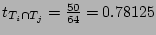
In this section, we evaluate the accuracy of the simple scheme in
estimating the fan-outs of sources and in detecting super sources.
Figure 8 compares the fan-outs of the sources
estimated using our simple scheme with the their actual fan-outs in
traces , , and respectively. In these experiments,
a flow sampling rate of  and a bit array of size and a bit array of size  bits is
used. The figure only plots the points whose actual fan-out values
are above 15 since lower values (i.e., bits is
used. The figure only plots the points whose actual fan-out values
are above 15 since lower values (i.e.,  ) are not interesting for
finding super sources.
The solid diagonal line in each figure denotes perfect estimation,
while the dashed lines denote an estimation error of ) are not interesting for
finding super sources.
The solid diagonal line in each figure denotes perfect estimation,
while the dashed lines denote an estimation error of  . The
dashed lines are parallel to the diagonal line since both x-axis and
y-axis are on the log scale. Clearly the closer the points cluster
around the diagonal, the more accurate the estimation is. We observe that
the simple scheme achieves reasonable accuracy for relatively large
fan-outs in all three traces. Figure 8 also
reflects the false positives and negatives in detecting super sources.
For a given threshold 50, the points that fall in ``Area I''
corresponds to false positives, i.e., the sources whose actual
fan-outs are less than the threshold but the estimated fan-outs are
larger than the threshold. Similarly, the points that fall in ``Area
II'' corresponds to false negatives, i.e., the sources whose
actual fan-outs are larger than the threshold but the estimated
fan-outs are smaller than the threshold. We observe that in
Figure 8, points rarely fall into Areas I and II (i.e., very few false
positives and negatives). . The
dashed lines are parallel to the diagonal line since both x-axis and
y-axis are on the log scale. Clearly the closer the points cluster
around the diagonal, the more accurate the estimation is. We observe that
the simple scheme achieves reasonable accuracy for relatively large
fan-outs in all three traces. Figure 8 also
reflects the false positives and negatives in detecting super sources.
For a given threshold 50, the points that fall in ``Area I''
corresponds to false positives, i.e., the sources whose actual
fan-outs are less than the threshold but the estimated fan-outs are
larger than the threshold. Similarly, the points that fall in ``Area
II'' corresponds to false negatives, i.e., the sources whose
actual fan-outs are larger than the threshold but the estimated
fan-outs are smaller than the threshold. We observe that in
Figure 8, points rarely fall into Areas I and II (i.e., very few false
positives and negatives).
While this scheme works well with 1/4 sampling rate, it cannot produce
good estimations with smaller sampling rates (e.g., 1/16. We omit the
experimental results here due to lack of space.).
However such lower sampling rates might be necessary to keep up
with very high link speeds such as 40 Gbps (OC-768).
We repeat the above experiment under the aforementioned second
definition of source and destination, in which the source label is
src_IP and destination label is dst_IP, dst_port.
Figure 9 plots the estimated fan-outs of
sources in trace IPKS+. With this definition the trace has
9,359 sources and 140,140 distinct source-destination pairs. We can
see from the figure that our estimation is also quite accurate with
this second definition of source and destination.
Figure 9:
Actual vs. estimated fan-out of
sources for trace with flow sampling rate 1/4. The
aforementioned second definition of source and destination labels is
used here. Note that both x-axis and y-axis are on logscale.
|
3 Accuracy of the advanced scheme
In this section we evaluate the accuracy of the advanced scheme using
both trace-driven simulation and theoretical analysis. The estimation
accuracy of the advanced scheme is a function of the various design
parameters, including the size and shape of the 2D bit array
(i.e., the number of rows and columns ) and the number of hash
functions ().
In the experiments we set the size of to 128KB (64 rows
 16,384 columns), and the flow sampling rate to 1.
This configuration is very space-efficient. For example it only uses
7 bits per flow on the average for the trace . 16,384 columns), and the flow sampling rate to 1.
This configuration is very space-efficient. For example it only uses
7 bits per flow on the average for the trace .
Figure 10:
Actual vs. estimated fan-out of sources by
the advanced scheme. Notice both axes are on logscale.
[trace IPKS+]
![\includegraphics[scale=0.4]{compare_hybrid_1.0.IPKS+.eps}](img173.png)
[trace UNC]
![\includegraphics[scale=0.4]{compare_hybrid_1.0.UNC.eps}](img174.png)
[trace USC]
![\includegraphics[scale=0.4]{compare_hybrid_1.0.USC.eps}](img175.png)
|
Figure 10 compares the fan-out values estimated using
the advanced scheme with the actual fan-outs of the corresponding
sources given three different traces.
Compared with the corresponding plots in Figure 8,
the points are much closer to the diagonal lines, which means that the
advanced scheme is much more accurate than the simple scheme.
In Figure 11, we repeat the experiments with
source and destination labels defined as src_IP and
dst_IP,dst_port, respectively. Compared with the result of
the simple scheme (Figure 9) the points are
much closer to the diagonal again, indicating the higher accuracy
achieved by the advanced scheme.
Note that in the experiments above we set the flow
sampling rate to instead of used in the experiments of the simple
scheme since as we described in Section 3.3 and
Section 4.4 respectively for a fully utilized OC-192
link the simple scheme requires flow sampling rate but the identity
sampling module of the advanced scheme can record  flow labels. flow labels.
The accuracy of the estimation can be characterized by the average
relative error of the estimator, which is equal to the standard
deviation of the ratio
 which can be
computed by Theorem 3. which can be
computed by Theorem 3.
Figure 12 shows the average relative error plotted against
estimated fan-outs for the sources in the trace . Experiments
on other traces produced similar results. The average relative error
shows a sharply downward trend when the estimated value of fan-out
increases in Figure 12. This is a very desirable property
as we would like our mechanism to be more accurate when estimating
larger fan-outs. Towards the right extreme of the figure, the average
relative error starts to increase. This is because the selected bit
vectors become almost full (``saturation'') when the fan-out value is
close to 266 (). As we discussed in
Section 4.3 the accuracy of our estimator would
degrade when the corresponding column vectors become
saturated. It does not affect the accuracy of our scheme for
detecting super sources, but to accurately estimate the exact fan-out
values that are large, the aforementioned multi-resolution
extension [6,11,12] is needed.
The accuracy of the estimator can also be characterized by the
probability of the estimated values
falling into the
interval
![$ [(1-\epsilon)F_s, (1+\epsilon)F_s]$](img182.png) , where is actual
fan-out of the source . This quantity can be numerically computed
by Monte-Carlo Simulation as follows. We first use the trace to
construct the 2D bit array (serving as ``background noise''). Then
we synthetically generate a source that has fan-out value and
insert it into by randomly selecting 3 different columns. The
estimator (Formula 6) is used to obtain the
. The above operations are repeated 100,000 times to
compute the probabilities shown in Figure 12. , where is actual
fan-out of the source . This quantity can be numerically computed
by Monte-Carlo Simulation as follows. We first use the trace to
construct the 2D bit array (serving as ``background noise''). Then
we synthetically generate a source that has fan-out value and
insert it into by randomly selecting 3 different columns. The
estimator (Formula 6) is used to obtain the
. The above operations are repeated 100,000 times to
compute the probabilities shown in Figure 12.
Figure 13 shows the plot of
 for different
values of , where for different
values of , where
![$ 1-\delta = Prob[(1-\epsilon)F_s \le \widehat{F_s} \le
(1+\epsilon)F_s]$](img184.png) . Each curve corresponds to a specific level of
relative error tolerance, i.e., a specific choice of . Each curve corresponds to a specific level of
relative error tolerance, i.e., a specific choice of  , and
represents the probability that the estimated value is within this
factor of the actual value. For example, the curve for , and
represents the probability that the estimated value is within this
factor of the actual value. For example, the curve for
 shows that around
  of the time the estimate is within of the time the estimate is within  of
the actual value. Notice how the curves in the figure have an upward
trend first and then show a downward trend as the fan-out increases
further. This corresponds exactly to the aforementioned ``saturation''
situation. of
the actual value. Notice how the curves in the figure have an upward
trend first and then show a downward trend as the fan-out increases
further. This corresponds exactly to the aforementioned ``saturation''
situation.
Figure 14:
Actual vs. estimated fan-out of sources by extension of the advanced scheme including deletions. Notice both axes are on logscale.
|
To evaluate the extension of the advanced scheme to estimate
outstanding fan-outs we use the pair of traces, and ,
collected simultaneously on both directions of a link. We extract all
the acknowledgment packets from to produce the 2D bit array
using the transposed update algorithm
(Figure 7). The same parameters are configured
for both 2D bit arrays and . Figure 14 shows
the scatter diagram of the fan-out estimated using our proposed scheme
( axis) vs. actual outstanding fan-out ( axis) vs. actual outstanding fan-out ( axis). The fact that
most points are concentrated within a narrow band of fixed width along
the diagonal line indicates that our estimator is accurate on
estimating outstanding fan-outs. axis). The fact that
most points are concentrated within a narrow band of fixed width along
the diagonal line indicates that our estimator is accurate on
estimating outstanding fan-outs.
7 Related work
The problem of detecting super sources and destinations has been
studied in recent years. In general, three approaches have been
proposed in the literature:
1. A straightforward approach is to keep track, for each source/destination,
the set of distinct destinations/sources that it contacts, using a hash table.
This approach is adopted in Snort [19] and FlowScan
[17]. It is straightforward to implement but
not memory-efficient, since most of the source-destination pairs in
the hash table do not come from super sources/destinations. As mentioned
before, this approach is not feasible for monitoring high-speed links
since the hash table typically can only fit into DRAM.
2. Data streaming algorithms are designed by Estan et
al. [6] mainly for estimating the number of active flows in
the Internet traffic.
However, it is stated in [6], that one variant of their
scheme, i.e., triggered bitmap, can be used for identifying the super
sources.
This algorithm maintains a small bitmap (4 bytes) for each source
(subject to hash collision), for estimating its fan-out. Once the
number of bits set in the small bitmap exceeds a certain threshold
(indicting a large fan-out), a large multi-resolution bitmap is
allocated to perform a more accurate counting of its fan-out. Since
the implementation of the binding between the source and the bitmap is
not elaborated in [6], we speculate that the binding is
implemented as a hash table, which can be quite costly if it has to
fit in SRAM (for high-speed processing). Also, its memory efficiency
is further limited by allocating at least 4 bytes for each source.
3. Recently Venkataraman et al. [20]
propose two flow sampling based techniques for detecting super
sources/destinations. Their one-level and two-level filtering
schemes both use
a traditional hash-based flow sampling technique for estimating
fan-outs. We explained in Section 3.1 that, when
this scheme is used for high-speed links (e.g., 10 or 40 Gbps), the
sampling rate is typically low due to the aforementioned traffic burst
problem. This prevents the algorithms from achieving high estimation
accuracy. In addition, the memory usage of both schemes, which
use hash tables, is much higher than our advanced scheme.
They only mentioned the possibility of replacing hash table with Bloom
filters to save space, but did not fully specify the details of the
scheme (e.g., parameter settings).
This makes a head-on comparison of our schemes with theirs very
difficult. In fact, after this replacement (of hash table with Bloom
filters), their scheme becomes a variant of Space Code Bloom Filter
(SCBF) we proposed in [12], with a slightly different
decoding algorithm.
Their decoding algorithm has similar computational complexity as that
of SCBF, which is an order magnitude more expensive than that of our
advanced scheme.
This may prevent our SCBF scheme (and their scheme as well) from
operating at very high link speeds (e.g., 40 Gbps).
8 Conclusion
Efficient and accurate detection of super sources and destinations at
high link speeds is an important problem in many network security and
measurement applications. In this work we attack the problem with a
new insight that sampling and streaming are often suitable for
capturing different and complementary regions of the information
spectrum, and a close collaboration between them is an excellent way
to recover the complete information. This insight leads to two novel
methodologies of combining the power of streaming and sampling,
namely, ``filtering after sampling'' and ``separation of counting and
identity gathering'', upon which our two solutions are built
respectively. The first solution improves the estimation accuracy of
hash-based flow sampling by allowing for much higher sampling rate,
through the use of a embedded data streaming module for filtering/smoothing the
bursty incoming traffic. Our second solution combines the power of
data streaming in efficiently retaining and estimating fan-out/fan-in
associated with a given source/destination, and the power of sampling
in generating a list of candidate source/destination identities.
Mathematical analysis and trace-driven experiments on real-world
Internet traffic show that both solutions allow for accurate detection
of super sources and destinations.
- 1
-
B. H. Bloom.
Space/time trade-offs in hash coding with allowable errors.
CACM, 13(7):422-426, 1970.
- 2
-
J. Carter and M. Wegman.
Universal classes of hash functions.
Journal of Computer and System Sciences, pages 143-154, 1979.
- 3
-
N. Duffield and M. Grossglauser.
Trajectory sampling for direct traffic observation.
IEEE transaction of Networking, pages 280-292, June 2001.
- 4
-
N. Duffield, C. Lund, and M. Thorup.
Estimating flow distribution from sampled flow statistics.
In Proc. ACM SIGCOMM, August 2003.
- 5
-
C. Estan and G. Varghese.
New Directions in Traffic Measurement and Accounting.
In Proc. ACM SIGCOMM, August 2002.
- 6
-
C. Estan and G. Varghese.
Bitmap algorithms for counting active flows on high speed links.
In Proc. ACM/SIGCOMM IMC, October 2003.
- 7
-
W. Fang and L. Peterson.
Inter-AS traffic patterns and their implications.
In Proc. IEEE GLOBECOM, December 1999.
- 8
-
N. Hohn and D. Veitch.
Inverting sampled traffic.
In Proc. ACM/SIGCOMM IMC, October 2003.
- 9
-
J. Jung, B. Krishnamurthy, and M. Rabinovich.
Flash crowds and denial of service attacks: Characterization and
implications for cdn and web sites.
In Proc. World Wide Web Conference, May 2002.
- 10
-
R. Karp, S. Shenker, and C. Papadimitriou.
A simple algorithm for finding frequent elements in streams and bags.
ACM Transactions on Database Systems (TODS), 28:51-55, 2003.
- 11
-
A. Kumar, M. Sung, J. Xu, and J. Wang.
Data streaming algorithms for efficient and accurate estimation of
flow size distribution.
In Proc. ACM SIGMETRICS, 2004.
- 12
-
A. Kumar, J. Xu, J. Wang, O. Spatschek, and L. Li.
Space-Code Bloom Filter for Efficient per-flow Traffic
Measurement.
In Proc. IEEE INFOCOM, March 2004.
- 13
-
R. Motwani and P. Raghavan.
Randomized Algorithms.
Cambridge University Press, 1995.
- 14
-
CISCO Tech Notes.
Cisco netflow.
available at https://www.cisco.com/warp/public/732/netflow/
index.html.
- 15
-
V. Paxon.
An analysis of using reflectors for distributed denial-of-service
attacks.
Computer Communication Review, 2001.
- 16
-
D. S. Phatak and T. Goff.
A novel mechanism for data streaming across multiple IP links for
improving throughput and reliability in mobile environments.
In Proc. IEEE INFOCOM, June 2002.
- 17
-
D. Plonka.
Flowscan: A network traffic flow reporting and visualization tool.
In Proc. USENIX LISA, 2000.
- 18
-
M. Ramakrishna, E. Fu, and E. Bahcekapili.
Efficient hardware hashing functions for high performance computers.
IEEE Transactions on Computers, pages 1378-1381, 1997.
- 19
-
M. Roesch.
Snort-lightweight intrusion detection for networks.
In Proc. USENIX Systems Administration Conference, 1999.
- 20
-
S. Venkataraman, D. Song, P. Gibbons, and A. Blum.
New streaming algorithms for fast detection of superspreaders.
In Proc. NDSS, 2005.
- 21
-
K.Y. Whang, B.T. Vander-zanden, and H.M. Taylor.
A linear-time probabilistic counting algorithm for database
applications.
IEEE transaction of Database Systems, pages 208-229, June
1990.
- 22
-
Y. Zhang, S. Singh, S. Sen, N. Duffield, and C. Lund.
Online identification of hierarchical heavy hitters: Algorithms,
evaluation, and application.
In Proc. ACM/SIGCOMM IMC, October 2004.
- 23
-
Q. Zhao, A. Kumar, J. Wang, and J. Xu.
Data streaming algorithms for accurate and efficient measurement of
traffic and flow matrices.
In Proc. ACM SIGMETRICS, June 2005.
- 24
-
Q. Zhao, A. Kumar, and J. Xu.
Joint data streaming and sampling techniques for detection of super
sources and destinations.
In Technical Report, July 2005.
Joint Data Streaming and Sampling Techniques for Detection of Super Sources and Destinations
This document was generated using the
LaTeX2HTML translator Version 2002-2-1 (1.70)
Copyright © 1993, 1994, 1995, 1996,
Nikos Drakos,
Computer Based Learning Unit, University of Leeds.
Copyright © 1997, 1998, 1999,
Ross Moore,
Mathematics Department, Macquarie University, Sydney.
The command line arguments were:
latex2html -split 0 -show_section_numbers -local_icons fanout.tex
The translation was initiated by Qi Zhao on 2005-08-09
Footnotes
- ... source
- Super sources have also been referred to
as ``superspreaders'' in literature [20].
- ... streaming
- As a note of clarification, the term
data streaming here has no connection with the transmission of
multimedia data known as media (audio and video) streaming
[16].
- ... sources.
- There is no explicit inversion procedure to recover the
number of flows if packet sampling is used. The technique used in
[4] may be helpful but does not provide accurate
answers.
- ...
table
- A small buffer in SRAM will not be able to smooth out
such bursts since at high link speeds, such bursts can easily fill up
several Megabytes of buffer in a matter of milliseconds.
- ...
counterparts.
- We can use multiple independent hash functions
to reduce the probability of collisions. But it will significantly
increases the overhead of updating and does not improve the
estimation result too much.
- ... attacks)
- Note that the worst case for
hash-based flow sampling is different. It occurs when a few of the
sampled flows contain most of the traffic on a link.
- ... Poisson
- The inter-arrival time is in fact
of geometric distribution.
- ... 128KB.
- We assume a conservative average
packet size of 1,000 bits, to our disadvantage. Measurements from
real-world Internet traffic report much larger packet sizes.
- ... independent
- Such hash functions
are referred to as -universal hash function in
literature [2]. It has been shown empirically
in [2] that the family of hash functions are very
close to -universal statistically when operating on real-world
data, for small values (e.g.,
 ). ).
- ... process
- Again, two ping-pong modules can be used in
an alternating fashion to avoid any operational interruption.
- ...
storage
- This is estimated based on the typical load
factor (defined later) we place on the bit vector.
- ... this.
-
Note that we do not show an example distribution for the
previous simple scheme since the estimator
of it
relies on where the flows with source appear in the packet stream, i.e.,
the values of when the flows arrive (cf. Formula 2).
Therefore the estimator may have different distributions given a fixed
value of .
- ... negatives
- One shall not simply compare this false positive
and negative ratios with the results in [20] since there only
when the scheme fails to detect a source whose fan-out is several (say 5) times larger
than the threshold will a false negative be declared.
- ...
saturated
- For more details about this please refer to
[21].
- ... algorithm
- In [12], we decode for the
exact value of the parameter to be estimated while their
scheme [20] decodes for a lower bound of the parameter.
Qi Zhao
2005-08-09
|

![\includegraphics[scale=0.4]{dist_new.eps}](img132.png)
![\includegraphics[scale=0.4]{compare_mve_0.25_other.IPKS+.eps}](img171.png)
![\includegraphics[angle=0, width=0.98\textwidth]{compare_hybrid_1.0_other.IPKS+.eps}](img177.png)
![\includegraphics[angle=0, width=0.98\textwidth]{err.ipks+.eps}](img178.png)
![\includegraphics[angle=0, width=0.98\textwidth]{prob.64.3.eps}](img180.png)
![\includegraphics[scale=0.4]{compare_del_1.0.eps}](img188.png)

![\includegraphics[scale=0.54]{sampling1.eps}](img19.png)
![% latex2html id marker 706
\framebox[3in][l]{
\begin{minipage}{3in}
{\noind...
...\hspace*{0.3in} /* The number of \lq\lq 0''s is decreased by 1 */
\end{minipage}
}](img20.png)
![$\displaystyle Var[\widehat{F_s}] \approx \frac{\sum_{j=1}^{pF_s}\frac{w-u_j}{u_j}}{p^2}+\frac{F_s(1-p)}{p}$](img55.png)
![\includegraphics[scale=0.55]{advanced.eps}](img57.png)
![\includegraphics[scale=0.5]{eg.eps}](img58.png)
![% latex2html id marker 1379
\framebox[3in][l]{
\begin{minipage}{3in}
{\noin...
...5in]
{\arabic{linecn}.}}\hspace*{0.3in} $A[row,col] := 1$\\
\end{minipage}
}](img59.png)
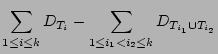
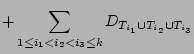
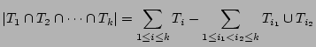
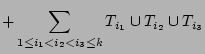
![$\displaystyle Var[\widehat{F_s}] \approx -m \sum_{i=1}^{3}f(t_{T_i}) - m \sum_{1 \le i_1 < i_2 \le 3}f(t_{T_{i_1} \cup T_{i_2}})\nonumber$](img126.png)
![% latex2html id marker 1636
\framebox[3in][l]{
\begin{minipage}{3in}
{\noinde...
....15in]
{\arabic{linecn}.}}\hspace*{0.4in} $B[row,col] := 1$\\
\end{minipage}
}](img148.png)