IMC '05 Paper
[IMC '05 Technical Program]
Optimal Combination of Sampled Network Measurements
Nick Duffield Carsten Lund Mikkel Thorup
AT&T Labs–Research, 180 Park Avenue, Florham Park, New Jersey,
07932, USA
{duffield,lund,mthorup}@research.att.com
|
Abstract
IP network traffic is commonly measured at multiple points in order
that all traffic passes at least one observation point. The
resulting measurements are subsequently joined for network analysis.
Many network management applications use measured traffic rates
(differentiated into classes according to some key) as their input
data. But two factors complicate the analysis. Traffic can be
represented multiple times in the data, and the increasing use
of sampling during measurement means some classes of traffic may be
poorly represented.
In this paper, we show how to combine sampled traffic
measurements in way that addresses both of the above issues.
We construct traffic rate estimators that combine data from
different measurement datasets with minimal or close to minimal
variance. This is achieved by robust adaptation to the estimated
variance of each constituent. We motivate the method with two
applications: estimating the interface-level traffic matrix in a
router, and estimating network-level flow rates from measurements
taken at multiple routers.
1 Introduction
1.1 Background
The increasing speed of network links makes it infeasible to collect
complete data on all packets or network flows. This is due to the costs and
scale of the resources that would be required to accommodate the data
in the measurement infrastructure. These resources are (i) processing
cycles at the observation point (OP) which are typically scarce in a
router; (ii) transmission bandwidth to a collector; and (iii)
storage capacity and processing cycles for querying and analysis at
the collector.
These constraints motivate reduction of the data. Of three classical
methods—filtering, aggregation and sampling—the first two require
knowing the traffic features of interest in advance, whereas only
sampling allows the retention of arbitrary detail while at the same
time reducing data volumes. Sampling also has the desirable property
of being simple to implement and quick to execute, giving it an
advantage over recently developed methods for computing compact
approximate aggregates such as sketches [14].
Sampling is used extensively in traffic measurement.
sFlow [17] sends packet samples directly to a
collector. In Trajectory Sampling, each packet is selected either at
all points on its path or none, depending on the result of applying
a hash function to the packet content [3]. In Sampled NetFlow
[1], packets are sampled before the
formation of flow statistics, in order to reduce the speed
requirements for flow cache lookup. Several methods
focus measurements on the small proportion of longer
traffic flows that contain a majority of packets.
An adaptive packet
sampling scheme for keeping flow statistics in routers which includes
a binning scheme to keep track of flows of different lengths is
proposed in [7]. Sample
and Hold [8] samples new flow cache instantiations, so
preferentially sampling longer flows. RATE [12] keeps
statistics only on those flows which present successive packets to the
router, and uses these to infer statistics of the original traffic.
Packet sampling methods are currently being standardized in the Packet
Sampling (PSAMP) Working Group of the Internet Engineering Task Force
[15].
Flow records can themselves be sampled within the measurement
infrastructure, either at the collector, or at intermediate staging
points. Flow-size dependent sampling schemes have been proposed
[4, 5, 6] to
avoid the high variance associated with uniform sampling of flows with
a heavy tailed length distribution.
1.2 Motivation
Multiple Traffic Measurements. This paper is motivated by
the need to combine multiple and possibly overlapping samples of
network traffic for estimation of the volumes or rates of matrix
elements and other traffic components. By a traffic component we mean
a (maximal) set of packets sharing some common property (such as a flow
key), present in the network during a specified time frame. Traffic
OPs can be different routers, or different interfaces on the same
router. Reasons for taking multiple measurements include: (i) all
traffic must pass at least one OP; (ii) measurements must be taken at
a specified set of OPs; and (iii) network traffic paths must be directly
measured.
Sampling and Heterogeneity. Traffic analysis often requires
joining the various measurement datasets, while at the same time
avoiding multiple counting. Sampling introduces further complexity
since quantities defined for the original traffic (e.g. traffic
matrix elements) can only be estimated from the samples. Estimation
requires both renormalization of traffic volumes in order to take
account of sampling, and analysis of the inherent estimator
variability introduced through sampling.
Depending on the sampling algorithm used, the proportion of traffic
sampled from a given traffic component may depend on (i) the sampling
rate (e.g. when sampling uniformly) and/or (ii) the proportion of that
component in the underlying traffic (e.g. when taking a fixed number
of samples from a traffic population). Spatial heterogeneity in
traffic rates and link speeds presents a challenge for estimating
traffic volumes, since a traffic component may not be well
represented in measurements all points, and sampling rates can
differ systematically across the network. For example, the sampling
rate at a lightly loaded access link may be higher than at a heavily
loaded core router. Changes in background traffic rates (e.g. due to
attacks or rerouting) can cause temporal heterogeneity in the
proportion of
traffic sampled.
Combining Estimates. This paper investigates
how best to combine multiple estimates of a given traffic
component. Our aim is to minimize the variability of the combined
estimate. We do this by taking a weighted average of the component
estimates that takes account of their variances. Naturally, this
approach requires that the variance of each component is known, or can
at least be estimated from the measurements themselves. A major
challenge in this approach is that inaccurate estimates of the
variance of the components can severely impair the accuracy of the
combination. We propose robust solutions that adapt to estimated
variances while bounding the impact of their inaccuracies.
What are the advantages of adapting to estimated variances, and
combining multiple estimates? Why not simply use the
estimate with lowest variance? The point of adaptation is that the
lowest variance estimate cannot generally be identified in advance, while
combining multiple estimates gains significant reduction in variance.
The component estimators are aggregates of individual measurements.
Their variances can be estimated provided the sampling parameters in
force at the time of measurement are known. This is possible when
sampling parameters are reported together the measurements, e.g., as
is done by Cisco Sampled NetFlow [2]. The
estimated variance is additive over the measurements. This follows
from a subtle but important point: we treat the underlying traffic as
a single fixed sample path rather than a statistical process. The only
variance is due to sampling, which can be implemented to be
independent over each packet or flow record. Consequently, variance
estimates can be aggregated along with the estimates themselves, even
if the underlying sampling parameters change during the period of
aggregation.
We now describe two scenarios in which multiple overlapping traffic
measurement datasets are produced, in which our methodology can be
usefully applied. We also mention a potential third application,
although we do not pursue it in this paper.
1.3 Router Matrix Estimation
Router Measurements and Matrix Elements. Applications such
as traffic engineering often entail determining traffic matrices,
either between ingress-egress interface pairs of a router, or at finer
spatial scales, e.g., at the routing prefix level or subnet level
matrices for traffic forwarded through a given ingress-egress
interface pair. A common approach to traffic matrix estimation is for routers to
transmit reports (e.g. packet samples or NetFlow statistics)
to a remote collector, where aggregation into matrix elements (MEs) is
performed.
Observation Points and Sampling Within a Router.
The choice of OPs within the
router can have a great effect on the accuracy of traffic
matrices estimated from samples. Consider the following alternatives:
-
Router-level Sampling: all traffic at the router is
treated as a single stream to be sampled. We assume ingress and
egress interface can be attributed to the measure traffic, e.g., as
reported by NetFlow.
- Unidirectional Interface-level Sampling: traffic is sampled
independently in one direction (incoming or outgoing) of each
interface.
- Bidirectional Interface-level Sampling: traffic is sampled
independently in both interface directions.
Comparing Sampling at the Observation Points.
Accurate estimation of an ME requires sufficiently many flows to be sampled from it.
For example, in uniform sampling with probability p, the relative
standard deviation for unbiased estimation of the total bytes of n
flows behaves roughly as ∼ 1/√np.
We propose two classes
of important MEs:
-
(i)
- Large matrix elements: these form a significant
proportion of the total router traffic.
- (ii)
- Relatively large matrix elements: these form a
significant proportion of the traffic on either or both of their ingress
or egress router interfaces. (We use the terms small
and relatively small in an obvious way).
Gravity Model Example. In this case the ME mxy from interface
x to interface y is proportional to Mxin Myout where
Min and Mout denote the interface input and output totals; see
[13, 18]. The large MEs mxy are those
for which both Mxin and
Myout are large. The relatively large MEs are those
for which either Mxin or
Myout (or both) are large.
Router level sampling is good for estimating large MEs, but not those
that are only relatively large at the router level. This is
because the sampling rate is independent of its ingress and
egress interfaces. In the gravity model, router sampling is good for
estimating the “large-to-large” MEs, (i.e. those mxy for which
both Mxin and Myout are large) but not good for estimating
“large-to-small” and “small-to-large” (and “small-to-small”)
MEs.
Unidirectional interface-level sampling offers some improvement, since
one can use a higher sampling rate on interfaces that carry less
traffic. However, unidirectional sampling, say on the ingress
direction, will not help in getting sufficient samples from a small
interface-to-interface traffic ME whose ingress is on an
interface that carries a high volume of traffic. In the
gravity model, “large-to-small” (and “small-to-small”) MEs would be problematic with ingress sampling.
Only bidirectional interface-level sampling can give a
representative sample of small but relatively large MEs. Two different estimates of the MEs could be formed,
one by selecting from an ingress interface all samples destined for a
given egress interface, and one by selecting from an egress interface
all samples from a given input interface. The two estimates are then
combined using the method proposed in this paper.
The effectiveness of router or interface level sampling
for estimating large or relatively large MEs
depends on the sampling rates employed and/or the resources
available for storing the samples in each case. If router level
and interface level sampling are employed, three
estimates (from router, ingress and egress sampling) can be combined.
In both the three-way and two-way combinations,
no prior knowledge is required of sampling parameters or the sizes of the
MEs or their sizes relative to the traffic streams from
which they are sampled.
Resources and Realization.
The total number of samples taken is a direct measure of the memory
resources employed. We envisage two realizations in which our
analysis is useful. Firstly, for router based resources, the question
is how to allocate a given amount of total router memory between
router based and interface based sampling.
The second realization is for data collection
and analysis. Although storage is far cheaper than in the router case,
there is still a premium on query execution speed. Record sampling
reduces query execution time. The question becomes how many samples
of each type (interface or router) should be used by queries.
1.4 Network Matrix Estimation Problem
The second problem that we consider is combining measurements taken at
multiple routers across a network. One approach is to measure at all
edge interfaces, i.e., access routers and peering points. Except
for traffic destined to routers themselves, traffic is sampled at both
ingress and egress to the network. Estimating traffic matrices between
edges is then analogous to the problem of estimating ingress-egress
MEs in a single router from bidirectional interface samples.
Once measurement and packet sampling
capabilities become standardized through the PSAMP and Internet
Protocol Flow Information eXport (IPFIX) [11] Working Groups
of the IETF, measurements could be ubiquitously
available across network routers. Each traffic flow
would potentially be measured at all routers on its path.
With today's path lengths, this might entail up to 30 routers
[16]. However, control of the total volume of data traffic
may demand that the sampling rate at each OP be quite low; estimates
from a single OP may be quite noisy. The
problem for analysis is how to combine these noisy estimates
to form a reliable one.
1.5 Parallel Samples
Multiple sampling methods may be used to match different applications
to the statistical features of the traffic. For example, the
distribution of bytes and packet per flow has been found to be
heavy-tailed; see [10]. For this reason, sampling flow
records with a non-uniform probability that is higher for longer flows
leads to more accurate estimation of the total traffic bytes than
uniform sampling; see [4]. On the other hand, estimates of
the number of flows are more accurate with uniform sampling. When
multiple sampling methods are used, it is desirable to exploit all
samples generated by both methods if this reduces estimator variance.
1.6 Outline
Section 2 describes the basic model for traffic
sampling, then describes a class of minimum variance convex
combination estimators. The pathologies that arise when using these
with estimated variance are discussed. Section 3 proposes
two regularized estimators
that avoid these pathologies. Section 4 recapitulates two
closely related sample designs for size dependent sampling of flow
records, and applies the general form of the regularized estimators
from Section 3 in each case. The remainder of the paper is
concerned with experimental evaluation of the regularized
size-dependent estimators for combining samples of flow
records. Section 5 evaluates their performance
in the router
interface-level traffic matrix estimation problem of
Section 1.3, and demonstrates the benefits of
including interface-level samples in the
combination. Section 6 evaluates performance
of the regularized estimators in the network matrix estimation problem
of Section 1.4 and shows how they provide a robust
combination estimates under wide spatial variation in the underlying
sampling rate. We conclude in Section 7.
2 Combining Estimators
2.1 Models for Traffic and Sampling
Consider n traffic flows labelled by i=1,2,…,n,
with byte sizes xi. We aim to estimate the byte total
X=Σi=1n xi.
Each flow i can be sampled at one of m
OPs, giving rise to estimators X1^,… Xm^ of X as follows. Let pij>0 be the probability that flow
i is selected at OP j. In general pij will be
a function of the size xi, while its dependence on j reflects the
possible inhomogeneity of sampling parameters across routers.
Let χij be the indicator of selection, i.e., χij=1
when the flow i is selected in measurement j, and 0
otherwise. Then each xij^=χijxi/pij is an unbiased
estimator of xi, i.e., E[xij^]=xi for all measurements
j. Renormalization by pij compensates for the fact that the
flow may not be selected. Clearly Xj^=Σi=1nxij^
is an unbiased estimator of X.
Note the xi are considered deterministic
quantities; the randomness in the Xi^ arises only from
sampling. We assume that the sampling decisions (the χij) for
each flow i at each of the m OPs are independent; it
follows that the Xj^ are independent.
2.2 Variance of Combined Estimators
In order to use all the information available concerning X, we
form estimators of X that depend jointly on the m estimators X1^,…,Xm^.
We focus on convex combinations of the Xj^,
i.e., estimators of the form
| |
X^ = |
|
λj Xj^, with |
λj∈[0,1], |
|
λj =1. (1) |
Each choice of the coefficients λ={λj: j=1,…,m} gives rise
to an estimator X^. Which λ should be used?
To evaluate the statistical properties of the estimators
(1), we focus on two properties: bias and
variance.
We now describe these for several cases of the
estimator (1). Let vj denote the variance Var(Xj^), i.e,
| |
vj= Var(Xj^)= |
|
Var(xij^)= |
|
|
|
(2) |
2.3 Average Combination Estimator
Here λj=1/m hence X^=m−1Σj=1m Xj^. This
estimator is unbiased since the λj are independent : E[X^]=Σj=1m λjE[Xj^]=X. It has variance Var(X^)=m−2Σj=1m vj. This estimator is very simple to
compute. However, it suffers from sensitivity of
Var(X^) to one constituent estimator Xj^ having large
variance vj, due to. e.g., a small sampling rate. The average estimator
is special case of the following class of estimator.
2.4 Independent {λj} and {Xj^}.
When λj is independent of Xj^,
X^ is unbiased, since
|
E[X^] = E[E[X^| |
|
]] = XE |
[ |
|
λj]=X
(3) |
| |
|
|
E |
[λi2]vj =
|
|
E[(λj−Λj( |
|
))2]vj + V0( |
|
)
(5) |
|
Λj( |
|
)= |
|
,
V0( |
|
)=1/ |
|
vj−1
(6) |
2.5 Estimators of Known Variance
For known variances vj, Var(X^) is minimized by
We do not expect the vi will be known a priori. For
general pij it is necessary to know all xi in order to
determine vi. However, in many applications, only the sizes xi
of those flows actually selected during sampling will be known.
We now mention two special cases in which the variance is at least
implicitly known.
2.6 Spatially Homogeneous Sampling
Each flow is sampled with the same probability at each
OP, which may differ between flows: pij=pi for some pi and all j.
Then the vi are equal and we take λj=Λj(v)=1/m. Hence
for homogeneous sampling, the average estimator from
Section 2.3 is the minimum variance convex combination of the
Xj^.
2.7 Pointwise Uniform Sampling
Flows are sampled uniformly
at each OP, although the sampling probability may vary
between points: pij=qj for some qj and all i.
Then
vj=(Σi=1n xi2)uj where uj=(1−qj)/qj.
The dependence of each vj in the {xi} is a common multiplier
which cancels out upon taking the minimum variance convex combination
X^ using
2.8 Using Estimated Variance
When variances are not know a priori, they may sometimes be estimated
from the data. For each OP j, and each flow i,
the random quantity
vij^ = χ ijxi2 (1− pij)/ pij2
(9)
is an unbiased estimator of the variance vij= Var(xij^) in
estimating xi by xij^. Hence
is an unbiased estimator of vj. Put another way, we add an amount xi2 (1−pij)/pij2 to the
estimator Vj^ whenever flow i is selected at observation
point j.
Note that Vj^ and Xj^ are dependent. This takes us
out of the class of estimators with independent {λj} and
{Xj^}, and there is no general simple form for the Var(X^) analogous to (4). An alternative is to estimate the
variance from an independent set of samples at each OP
j. This amounts to replacing χij by an independent identically distributed sampling
indicator {χ'ij} in (9). With this change,
we know from Section 2.4 that using
will result in an unbiased estimator
X^ in (1). But the estimator will not in general have
minimum possible variance V0(v) since λj is not
necessarily an unbiased estimator of Λj(v).
2.9 Some Ad Hoc Approaches
A problem with the foregoing is that an estimated variance Vj^
could be zero, causing Λj(V^) to be undefined.
On the other hand, the average
estimator is susceptible to the effect of high variances. Some ad hoc
fixes include:
AH1: Use λj=Λj(V^) on the subset of sample sets j
with non-zero estimated variance. If all estimated variances are
zero, use the average estimator.
AH2: Use the non-zero estimate of lowest estimated variance.
But these
estimators still suffer from a potentially far more serious pitfall:
the impact of statistical fluctuations in small estimated variances.
This is discussed further in Section 2.10.
2.10 Discussion
Absence of Uniformity and Homogeneity.
We have seen in Section 2.6 that the average estimator is
the minimum variance convex combination only when sampling is
homogeneous across OPs. In Section 2.7
we saw that we can form a minimum variance estimator without direct
knowledge of estimator variance only when sampling is uniform. In
practice, we expect neither of these conditions to hold for network
flow measurements.
Firstly, sampling rates are likely to vary
according to monitored link speed, and may be dynamically altered in
response to changes in traffic load, such as those generated by
rerouting or during network attacks. In one proposal,
[7], the sampling rate may be routinely changed on short
time scales during measurement, while the emerging PSAMP standard is
designed to facilitate automated reconfiguration of sampling rates.
Secondly, the recognition of the concentration of traffic in heavy
flows has led to sampling schemes in which the
sampling probability of a flow (either of the packets that constitute
it, or the complete flow records), depends on the flow's byte size
rather than being uniform; see [4, 5, 6, 8, 12].
Finally, in some sampling schemes, the effective sampling rate for an
item is a random quantity that depends on the whole set of
items from which it is sampled, and hence varies when different sets
are sampled from. Priority sampling
is an example; see Section 4.
Pathologies of Small Estimated Variances.
Using estimated variances brings serious pitfalls. The most
problematic of these is that samples taken with a low sampling rate
may have estimate variance close to or even equal to zero. Even if
the zero case is excluded in ad hoc manner, e.g. as described in
Section 2.9, a small and unreliable sample may spuriously
dominate the estimate because its estimated variance happens to be
small. Some form of regularization is required in order to
alleviate this problem. A secondary issue for independent variance
estimation is the requirement to maintain a second set of samples, so
doubling resource requirements.
In the next sections we propose a regularization for variance
estimation in a recently proposed flow sampling scheme that controls
the effect of small estimated variances, even in the dependent case.
3 Regularized Estimators
We propose two convex combination estimators
of the type (1) using random coefficients {λj}
of the form (11) but regularizing or bounding the
variances to control the impact of small estimated variances.
Both estimators take the form Σj λj Xj^ with λj=Λj(U^) for some estimated
variances U^, while they differ in which U^ is
used.
Both estimators are characterized by the set of quantities τ,
where for each OP j:
The τj may be known a priori from a given
functional dependence of pij on xi, or it may only be known
from the measurements themselves.
3.1 Regularized Variance Estimator
The first estimator ameliorates the impact of small underestimated
variances, while still allowing combination to take account of
different but well-estimated variances. Note that the estimated
variance vij^ obeys the bound
vij^ ≤ χijτj2
(13)
This suggests that we can
ameliorate the effects of random exclusion of a flow from a sample
by adding a small multiple s of τj2 to each variance estimator
Vj^. This represents the scale of uncertainty in variance
estimation. The addition has little effect when the estimated
variance arises from a large number of samples, but tempers the effect
of a small sample for which the variance happens to be small or even
zero. With this motivation,
the regularized variance estimator is X^ = Σj
λj Xj^ with
|
λj=Λj( |
|
) where
V'j^ = Vj^ + sτj2 (14) |
3.2 Bounded Variance Estimator
The second estimator uses a similar approach on the actual variance
vij, which obeys the bound:
If this bound were equality, we would then have Vj=Xτj, in
which case, the minimum variance estimator would be the
bounded variance estimator, namely, X^ = Σj
λj Xj^ with λj=Λj(Xτ) =
Λ(τ). The corresponding variance estimate for this
convex combination is V^ = Σj=1m λj2 Vj^.
The strength of this approach is that the variance estimate can take
account of knowledge of inhomogeneity in the sample rates (as
reflected by inhomogeneity in the τj) while not being subject to
statistical fluctuations in variance estimates.
Uniform and Homogeneous Sampling.
Note that uniform and homogeneous sampling fall into this
framework already (with equality in (15)), since in both
cases the dependence of the variances vj on the objects xi to be
sampled is a common factor over all OPs j, which
is hence eliminated from the coefficients λj.
Small Sampling Probabilities.
The tightness of the bound (15) depends on the functional
form of pij. One particular case is when sampling probabilities
are small. For this case we propose a linear approximation:
pij = xi/τ j + O( ( xi/τ j) 2)
(16)
This yields approximate equality in (15), provided all
xi are small compared with τj. We give an example of a sample
design with this property in Section 4.
3.3 Confidence Intervals
We form approximate conservative
confidence intervals for X^ by applying a regularization of the
type (14).
Thus the upper and lower confidence intervals are
X±^= X^ ± s ( V^ + sτ 2) (17) where s is the
target number of standard deviations away from the mean.
4 Size Dependent Flow Sampling
The remainder of the work in this paper will focus on two closely
related schemes for sampling completed flow records. These are
threshold sampling [4] and priority sampling
[6]. We briefly recapitulate these now.
4.1 Threshold Sampling
For a threshold z>0,
a flow of size x is sampled with probability pz(x)=min{1,x/z}.
Thus flows of size x≥ z are always
sampled, while flows of size x<z are sampled with probability
proportional to their size. This alleviates the problem of uniform
sampling, that byte estimation can have enormous variance due to
random selection or omission of large flows. In threshold sampling,
all flows of size at least z are always selected.
Starting with a set of flows with sizes {xi} as before, we form
an unbiased estimator X^ of X=Σi=1n xi using the
selection probabilities pi=pz(xi). (In this section we
suppress the index j of the OP). The estimator of X
from a single OP takes the form
X^ takes the specific form
| |
X^= |
|
χi xi/pz(xi)= |
|
χi max{xi,z} (18) |
Threshold sampling is optimal in the sense that it
minimizes the cost Cz= Var(X^)+z2N where N=Σi=1npi
is the expected number of samples taken. This cost expresses the
balance between the opposing goals of reducing the number of samples
taken, and reducing the uncertainty in estimating X. The value of
z determines the relative importance attached to these goals.
Applying the general formula (2), the variance of the estimate
X^ from a single OP is
| Var(X^)= |
|
xi max{z−xi,0} (19) |
| V^ = |
|
χi z max{z−xi,0} (20) |
4.2 Priority Sampling
Priority sampling provides a way to randomly select exactly k of the
n flows, weighted by flow bytes, and then form an unbiased estimator
of the total bytes X. The algorithm is as follows. For each flow
i, we generate a random number αi uniformly distributed in
(0,1], and construct its priorities zi^=xi/αi. We
select the k flows of highest priority. Let z'^ denote the
(k+1)st highest priority. At a single OP,
we for the estimate
of the total bytes X. Here χi is the indicator that flow i is
amongst the k flows selected. X^
is unbiased; see [6].
For priority sampling, the variance of X^ takes a similar form
to that of threshold sampling:
| Var(X^)= |
|
xi E[max{z'^−xi,0}] (22) |
| V^ = |
|
χi z'^ max{z'^−xi,0} (23) |
In priority sampling, inhomogeneity between observation
points arises not only through inhomogeneity of the number of flows
k selected, but also through the background traffic. Typically we
want to estimate the total bytes not of all sampled flows, but only of
a selection of them that share some property of interest, e.g., a
specific source and destination. The probability that a given
interesting flow will be amongst the k flows selected, depends also
on the sizes of all flows in the background traffic, which generally
varies between different OPs. Threshold sampling is independent
between flows.
4.3 Threshold and Priority Compared
The estimator (21) appears quite similar to that for
threshold sampling (18), except that the role of the
threshold z is played by the random quantity z'^. In fact, the
relationship is deeper: one can show that, conditioned on the
threshold z'^, the selection probabilities for each flow minimize
a cost analogous to Cz.
For applications, we see that threshold sampling is well suited to
streaming applications when buffer space is expensive (e.g., at a
router) since each object is sampled independently. Priority sampling
is able to constrain the number of samples taken, at the cost of
maintaining a buffer of k candidate samples during selection. It is
well suited to applications where buffering is less expensive (e.g.,
in a data aggregator or database)
4.4 Regularized Variance Estimators
Threshold and priority sampling both give rise to regularized
estimators as described in Section 3. Consider first
threshold sampling and let zj be the sampling threshold in force at
OP j. Then the quantity τj in
(12) is just zj. Moreover, pij is approximately
linear in xi, the sense of (16), and hence the bounded
variance estimator is expected to perform reasonably for flows whose
size xi are small compared with the zj. For priority sampling,
we use the random thresholds z'j in place of the zj. Although
this introduces additional variability; in practice priority
approximates threshold sampling closely for large number of samples.
In the next sections we show this heuristic performs well in experiments.
| |
|
1 |
2 |
3 |
4 |
5 |
6 |
7 |
8 |
| |
|
0.0004 |
0.04 |
0.1 |
0.004 |
0.03 |
0.8 |
0.02 |
0 |
| 1 |
0 |
0 |
0 |
0 |
0 |
0 |
0 |
0 |
0 |
| 2 |
0.5 |
8e-05 |
0 |
0.0007 |
0 |
0 |
0.5 |
0.0001 |
0 |
| 3 |
0.01 |
7e-05 |
0.0002 |
0 |
0 |
0.001 |
0.01 |
0.0004 |
0 |
| 4 |
0 |
0 |
0 |
0 |
0 |
0 |
0 |
0 |
0 |
| 5 |
0.2 |
2e-05 |
0 |
0.05 |
0.003 |
3e-05 |
0.1 |
0.006 |
0 |
| 6 |
0.3 |
0.0002 |
0.04 |
0.08 |
0.001 |
0.02 |
0.2 |
0.01 |
0 |
| 7 |
0.01 |
2e-05 |
0.003 |
0.0004 |
5e-06 |
0.006 |
0.0007 |
3e-05 |
0 |
| 8 |
1e-06 |
1e-06 |
0 |
0 |
0 |
0 |
0 |
0 |
0 |
Table 1: Router matrix elements for campus, with row and column sums, normalized
by total bytes
5 Experiments: Router Matrix
This section applies our method to traffic
measurement at routers.
As discussed in Section 1.3, while router level
sampling captures large MEs accurately, interface level sampling
offers the opportunity to accurately sample not just the relatively
large ones MEs, i.e., the largest amongst those seen at each
interface. This is particularly important for a method such as
priority sampling where, in order to provide a hard constraint on the use
of measurement resources, only a fixed number of samples are taken in
a given time period, There is a trade-off: if all resources were
deployed for interface sampling, then not all larger flows on some
heavily used interfaces might be sampled.
This motivates using a combined estimator. In this application we
explicitly want to take account of estimated variance, so we
use the regularized variance estimator of Section 3.
In experiments
using real flow data taken at two routers, we find that:
(i) For a given total number of samples, the regularized estimator
is more accurate than its individual consistent estimators or
averages thereof.
(ii) The regularized estimator is more accurate than the ad hoc
estimator AH1 when estimation error is large.
5.1 Router Data and Traffic Matrices
The data from this experiment comprised sampled NetFlow records
gathered from two routers in a major ISP network. These record
the total bytes of the sampled flow packets,
and the router input and output interfaces traversed by the flow.
Thus, it is possible to map each flow onto the appropriate router to
router traffic matrix.
The first dataset, campus comprises 16,259,841 NetFlow records
collected from a backbone router in a
corporate intranet during 24 hour period.
The active flow timeout was 30 minutes.
The maximum size was 3.94 GB and average size 20.4 kB. The router had 8
interfaces. Table 1 shows the interface MEs for a 10 minute period,
normalized by total bytes. Note the non-zero MEs range
over six orders of magnitude.
The second dataset, distribution comprises 1,765,477 NetFlow
records collected during 1 hour from a distribution router in an ISP
network. The active flow timeout was 1 minute, with maximum
flow size 3.97 MB and average 1.4 kB. The router had 236 interfaces
(and subinterfaces), whose line rates ranged from 622 MBps (OC-12)
down to 1.5 Mbps (T1). Only 1971 MEs are
non-zero. We represent these in Figure 1, where the
interfaces have been sorted in decreasing order of total input and
output bytes in the 1 hour period. The distribution of traffic per
interface is highly skewed: the busiest interface carries 46% of the
bytes, while the 10 busiest together carry 94%.
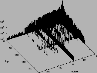
Figure 1: Matrix Elements of Dataset distribution. Interfaces are
ordered by total bytes
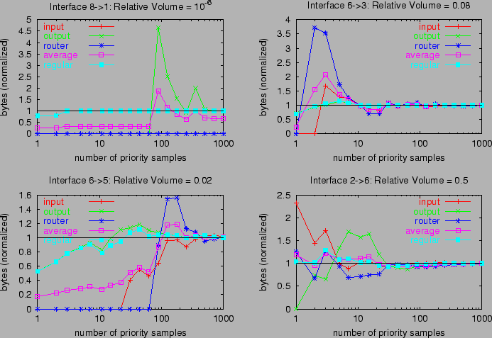
Figure 2: Estimator Comparison: input, output, router, average i,o,r
and regular i,o,r, for 4 matrix elements from Table 1
representing various relative volumes of the total bytes.
5.2 Notation for Estimators
input and output denote the byte estimators derived
input and output interface samples respectively, while
router denote the estimator derived from all flows
through the router, undifferentiated by interface. average i,o,r averages
input, output and router,
while average i,o averages only input and output. adhoc i,o,r combines the
estimators input, output and router as described in AH1
of Section 2.9, while regular i,o,r is the corresponding
regularized variance estimator from Section 3. bounded
is the bounded variance estimator. In priority sampling,
regular i,o,r(ki,ko,kr) denotes the regularized estimator in which
ki and ko priority samples were taken and each input and output
interface respectively, and kr were taken at the router level.
A Sample Path Comparison.
We compare the performance of the various estimators on several of the
campus MEs from Table 1, as a function of the number of
priority samples k per interface direction. The estimated MEs (normalized through
division by the true value) are displayed in Figure 2 for
k roughly log-uniformly distributed between 1 and 1000.
Perfect estimation is represented by the value 1. In this
evaluation we selected all flows contributing to a given ME, then progressively accumulated the required numbers k of
samples from the selection. For this reason, the variation with k is
relatively smooth.
There are N=8 interfaces. Each of the single estimators
was configured using the same number of
sample slots, i.e., input(k), output(k) and router(2Nk).
We compare these first; see Figure 2.
For the smaller MEs (8→1, 6→3 and 6→5),
input and output are noticeably more accurate than router: the relatively large MEs are better sampled at the
interface level than at the router level. average i,o,r(k,k,2Nk) performs poorly
because of the contribution of router, and also because it
driven down by the zero estimation from input and output
when the number of samples k is small; see, e.g., the 8→1 ME. Only for a large ME (2→6, constituting about half the traffic in the router)
does router accuracy exceed the worst of the interface methods.
Consequently, the accuracy of average i,o,r is better in this case too.
When there are noticeable differences between
the three single estimators, regular i,o,r(k,k,2Nk)
roughly follows the most accurate one. In the 2→6
ME, regular i,o,r follows input
most closely while in the 6→ 3 and 6→5 MEs, it follows
output.
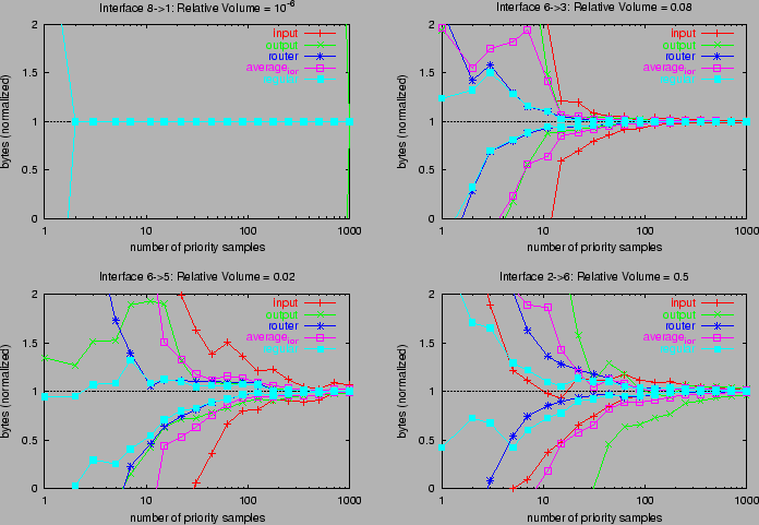
5.3 Confidence Intervals
Recall that each estimation method
produces and estimate of the
variance of the ME estimator. This was used to form upper and lower confidence
intervals in Section 3.3.
Figure 3 shows upper and lower confidence limits for
estimating the MEs of campus using the same router
interfaces as in Figure 2. These use (17) with
standard deviation parameter s=2.
8→1 is a special case. input has no estimated
error when k≥ 2. As can be seen from Table 1, 8→1 is the
only ME with ingress at interface 8. It comprises 2
flows, so the estimated variance and sampling
threshold are 0 for k≥ 2. The other methods perform poorly
(their confidence bounds are off the chart), since neither
output nor router samples this very small flow.
regular i,o,r displays the best overall performance in
Figure 2, i.e., it tends to have the smallest divergence
from the true value. Figure 3 show that the estimated
estimator variance tends to be the smallest too, giving narrower
confidence intervals than the other methods.
Figure 3: Comparing Confidence Intervals by method, for 4 matrix elements from Table 1
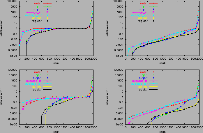
Figure 4: Relative Errors of Matrix Elements for Different
Estimators, Ranked by Size. Left: raw relative errors. Right: scaled relative
errors.
Top: 16 slots per
interface. Bottom: 128 slots per interface.
Estimator Accuracy for Fixed Resources.
Now we perform a more detailed comparison of the estimators with the
distribution dataset, using constant total sampling slots across
comparisons. The router has N=236 interfaces, each
bidirectional. For a given number k of sampling slots per interface
direction, we compare router(4Nk), input(4k),
output(4k), average i,o,r(k,k,2Nk), average i,o(2k,2k), adhoc i,o,r(k,k,2Nk)
and regular i,o,r(k,k,2Nk).
For k values of 16 and 128, and each estimation method, we sorted
the relative errors for each ME in increasing order, and
plotted them as a function of rank in the left
hand column of Figure 4. (The average flow sampling rates are
approximately 1 in 234 for k=16 and 1 in 30 for k=128).
The curves
have the following qualitative features. Moving from left to right,
the first feature, present only in some cases, is when the
curves start only at some positive rank, indicating all MEs up to that rank have been estimated either with
error smaller than the resolution 10−5.
The second feature is a curved portion of
relative errors
smaller than 1. The third feature is
a flat portion of relative errors, taking the value 1 for the
individual, adhoc i,o,r and regular i,o,r methods, and 1/2 and 1/3 for
average i,o and average i,o,r respectively. This happens when a ME
has no flows sampled by one of the individual estimators.
The final feature at the right hand side
are points with relative errors ε>1, indicating MEs
that have been overestimated by a factor ε+1.
We make the following observations:
(i) Interface sampling (input and output) and regular i,o,r and
adhoc i,o,r are uniformly more accurate that average i,o,r or router.
(ii) Interface sampling performs better than adhoc i,o,r or
regular i,o,r when errors are small. When an ME is very well estimated on a given interface, any
level information from another interface makes the estimate
worse. But when the best interface has a large estimation error, additional information can help reduce it: regular i,o,r and adhoc i,o,r
become more accurate.
(iii) The average-based methods perform poorly; we have argued that they are
hobbled by the worst performing component. For example, average i,o
performs worse than input and output since typically only one of these
methods accurate for a relatively large ME.
(iv) regular i,o,r and adhoc i,o,r have similar performance, but when there
are larger errors, they are worse on average for adhoc i,o,r.
(v) As expected, estimation
accuracy increases with the number of samples k, although
average i,o and average i,o,r are less responsive.
Although these graphs show that regular i,o,r and adhoc i,o,r are more
accurate than other estimators, is it not immediately evident that
this is due to the plausible reasons stated earlier, namely, the more
accurate inference of relatively larger flows on smaller
interfaces. Also it is not clear the extent to which interface
sampling can produce sufficiently accurate estimates at reasonable
sampling rates. For example, for k=128 (roughly 1 in 30 sampling of
flow records on average) about 25% of the MEs have
relative errors 1 or greater. We need to understand which MEs are
inaccurately estimated.
To better make this attribution we calculate a scaled
version of a MEs as follows. Let Q denote the set of
interfaces, and let mxy denote the
generic ME from interface x to interface y. Let
Min and Mout denote the interface input and output totals, so
that Mxin =Σy∈ Qmxy and Myout = Σx∈
Qmxy. If eyx is the relative error in estimating mxy
then we write the scaled version as
e'xy = exy max{ mxy/Mxin, mxy/Myout}
(24)
Here mxy/Mxin and mxy/Myout are the fractions of the
total traffic that mxy constitutes on it input and output
interfaces. Heuristically, e'xy deemphasizes errors in estimating
relatively
small
MEs.
We plot the corresponding ordered values of the errors e'xy in
the right hand column of Figure 4. Note:
(i) regular i,o,r and adhoc i,o,r are uniformly more accurate than other methods,
except for low sampling rates and low estimation errors, in which
case they perform about the same as the best of the other methods;
(ii) the accuracy advantage of regular i,o,r and adhoc i,o,r is more
pronounced at larger sampling rates;
(iii) regular i,o,r and adhoc i,o,r
display neither the third nor fourth features described above, i.e.,
no flat portion or errors greater than 1. This indicates that these
methods are successful in avoiding larger estimation errors for
the relatively large MEs, while for the other methods some
noticeable fraction of the relatively large MEs are badly estimated.
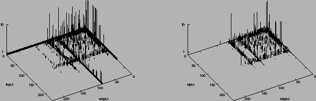
Figure 5: Matrix of relative errors. k=128 samples per interface
direction. Left: average i,o. Right: regular i,o,r.
We can also get a picture of the relative performance of the methods by
looking at the larger estimation errors of the whole traffic
matrix. As examples, we show in Figure 5
unscaled relative errors for k=128
samples per interface direction, for average i,o and regular i,o,r. Errors have
been truncated at 10 in order to retain detail for smaller
errors. Observe:
(i) average i,o is poor at estimating many MEs through the
largest interface (labeled 1) since smaller MEs are
poorly sampled at that interface. regular i,o,r performs better because
it uses primarily the estimates gathered at the other interface
traversed by these MEs.
(ii) regular i,o,r has a smaller number of large relative errors than
average i,o.
In order to get a broader statistical picture we repeated
the experiments reported in
Figure 4 100 times, varying the seed for the
pseudorandom number generator that governs random selection in
each repetition. The ranked root mean square (RMS) of the relative
errors shows broadly the same form as
Figure 4, but with smoother curves due to
averaging over many experiments.
6 Experiments: Network Matrix
In this section we shift the focus to combining a large
number of estimates of a given traffic component. Each estimate may
individually be of low quality; the problem is to combine them into a
more reliable estimate. As mentioned in Section 1.4, this
problem is motivated by a scenario in which routers or other network
elements ubiquitously report traffic measurements. A traffic
component can generate multiple measurements as it transits the
network.
A challenge in combining estimates is that they may be formed from
sample sets drawn with heterogeneous sampling rates and hence the
estimates themselves may have differing and unpredictable
accuracy, as described in Section 2.10.
For this reason, the approach of Section 3 is appealing, since
estimation requires no prior knowledge of sampling rates; it only
assumes reporting of the sampling rate in force when the sample was
taken.
6.1 Experimental Setup
We wished to evaluate the combined estimator from independent samples
of a traffic stream from multiple points. Since we do not have
traces taken from multiple locations, we used instead multiple
independent samples sets of the campus flow trace, each set
representing the measurements that would be taken from a single OP.
We took 30 sample sets in all, corresponding to the current maximum
typical hop counts in internet paths [16].
The experiments used threshold sampling, rather than
priority sampling, since this would have required the additional
complexity of simulating background traffic for each observation
point. Apart from packet loss or the possible effects of
routing changes, the multiple independent samples correspond with
those obtained sampling the same traffic stream at multiple points in
the network.
Our evaluations used multiple experiments, each of which
represented sampling of a different set of flows in the network. The
flow sizes were taken from successive portions
of the campus
trace (wrapping around if necessary), changing the seed
pseudorandom
number generator used for sampling in each experiment.
The estimates based on each set of independent samples were combined
using the following methods: average, adhoc, bounded and
regular. As a performance metric for each method,
we computed the
root mean square (RMS)
relative estimation error over 100 experiments.
| threshold |
adhoc |
bounded |
regular |
| 103 |
0.0017 |
0.0016 |
0.0017 |
| 104 |
0.0121 |
0.0066 |
0.0117 |
| 105 |
0.1297 |
0.0353 |
0.0883 |
| 106 |
0.4787 |
0.1293 |
0.3267 |
| 107 |
8.080 |
0.515 |
0.527 |
| 108 |
46.10 |
1.464 |
0.923 |
| 109 |
108.7 |
3.581 |
1.926 |
Table 2: Homogeneous Sampling. RMS relative error; 1000 flows, 30 sites
|
| threshold |
adhoc |
bounded |
regular |
| 103 |
0.00002 |
0.00002 |
0.00002 |
| 104 |
0.00012 |
0.00012 |
0.00012 |
| 105 |
0.00064 |
0.00063 |
0.00064 |
| 106 |
0.00340 |
0.00321 |
0.00339 |
| 107 |
0.01505 |
0.01110 |
0.01469 |
| 108 |
0.16664 |
0.05400 |
0.11781 |
| 109 |
0.78997 |
0.17387 |
0.37870 |
Table 3: Homogeneous Sampling. RMS relative error; 100,000 flows, 30 sites
|
6.2 Homogeneous Sampling Thresholds
As a baseline we used a uniform sampling threshold
at all OPs. In this case that bounded reduces to average. In 7
separate experiments we use a sampling threshold of 10i Bytes for
i=3,…,9. This covers roughly the range of flow sizes in the
campus dataset, and hence includes the range of z values that
would likely be configured if flow sizes generally conformed to the
statistics of campus. The corresponding sampling rate (i.e. the
average proportion of flows that would be selected) with threshold z
is π(z)=Σi min{1,xi/z}/N where {xi:i=1,…,N} are
the sizes of the N flows in the set. For this dataset π(z)
ranged from π(103)=0.018 to π(109)=1.9× 10⁻⁵.
We show a typical single path of the byte estimate (normalized by the
actual value) for a single experiment in
Figure 6.
This was for 10,000 flows sampled with
threshold 10MB at 100 sites. There were typically a handful of flows
sampled at each OP. The bounded estimate
relaxes slowly towards the true value. regular also follows at a
similar rate, but displays some bias. adhoc displays systematic
bias beyond 30 combinations. The bias strikingly shows the need for
robust estimation methods of the type proposed in this paper.
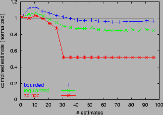
Figure 6: Combined estimators acting cumulatively over 100 independent estimates.
Summary RMS error statistics over multiple experiment are shown in Tables
2 and 3. Here we vary the number of
flows in the underlying population (1000 or 100,000) for 30
measurement sites. (Results for 10 measurement sites are not displayed
due to space constraints). bounded has
somewhat better performance than regular and significantly better
performance than adhoc. The differences are generally more
pronounced for 30 sites than for 10, i.e., bounded is able to take
the greatest advantage (in accuracy) of the additional
information. On the basis of examination of a number of individual
experiments of the type reported in Figure 6, this
appears to be due to lower bias in bounded.
6.3 Heterogeneous Sampling Thresholds
To model heterogeneous sampling rates we used 30 sampling thresholds
in a geometric progression from 100kB to 100MB, corresponding to average
sampling rates of from 0.016 to 8.9× 10⁻⁵. This range of z
values was chosen to encompass what we expect would be a range of
likely operational sampling rates, these being quite small in order to
achieve significant reduction in the volume of flow records through
sampling.
We arranged the thresholds in increasing order
105B=z1<…<zi<…<z30=108B, and for each m
computed the various combined estimators formed
from the m individual estimators obtained from
samples drawn using the m lowest thresholds
{zi:i=1,…,m}. The performance on traffic streams comprising
10,000 flows is shown in Figure 7. Qualitatively
similar results were found with 1,000 and 100,000 flows.
The RMS error of average initially decreases with path
length as it combines the estimators of lower variance (higher
sampling rate). But it
eventually increases as it mixes in estimators or higher variance
(lower sampling rate). RMS errors for bounded and regular are
essentially decreasing with path length, with bounded having
slightly better accuracy. The minimum RMS errors (over all
path lengths) of the three methods a roughly the same. Could
average be adapted to select and include only
those estimates with low variance? This would require an
additional decision of which estimates to include, and the best
trade-off between accuracy and path length is not known a priori. On
the other hand, bounded and regular can be used with all
available data, even with constituent estimates of high variance,
without apparent degradation of accuracy.
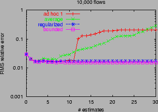
Figure 7: Heterogeneous Sampling Rates. RMS relative errors for
adhoc, average, regular and bounded, as a function of
number of estimates combined.
7 Conclusions
This paper combines multiple estimators of traffic volumes formed
from independent samples of network traffic. If the variance of
each constituent is known, a minimum variance convex combination
can be formed. But spatial and
temporal variability of sampling parameters mean that variance is best
estimated from the measurements themselves. The convex
combination suffers from pathologies if used naively with estimated variances.
This
paper was devoted to finding remedies to these pathologies.
We propose two regularized estimators that avoid the pathologies
of variance estimation. The regularized variance
estimator adds a contribution to estimated variance representing the
likely sampling error, and hence ameliorates the pathologies of estimating
small variances while at the same time allowing more reliable
estimates to be balanced in the convex combination estimator. The
bounded variance estimator employs an upper bound to the variance
which avoids estimation pathologies when sampling probabilities are
very small.
We applied our methods to two networking estimation problems:
estimating interface level traffic matrices in routers, and combining
estimates from ubiquitous measurements across a network.
Experiments with real flow data
showed that the methods exhibit: (i)
reduction in estimator variance, compared with individual
measurements; (ii) reduction in bias and estimator variance,
compared with averaging or ad hoc combination methods; and
(iii) application across a wide range of inhomogeneous sampling
parameters, without preselecting data for accuracy.
Although our experiments focused on
sampling flow records, the basic method can be used to
combine estimates derived from a variety of sampling techniques,
including, for example,
combining mixed estimates formed from uniform and non-uniform sampling
of the same population.
Further work in progress examines the
properties of combined estimators at an analytical level, and yields a deeper understanding
of their statistical behavior beyond the mean
and variance.
References
[1]- Random Sampled NetFlow. Cisco Systems.
http://www.cisco.com/univercd/cc/td/doc/product/software/ios123/123newft/123t/123t_2/nfstatsa.pdf
- [2]
-
Cisco IOS NetFlow Version 9 Flow-Record Format.
http://www.cisco.com/warp/public/cc/pd/iosw/prodlit/tflow_wp.htm#wp1002063
- [3]
-
N. G. Duffield and M. Grossglauser,
“Trajectory Sampling for Direct Traffic Observation”,
IEEE/ACM Transactions on Networking, vol. 9, pp. 280-292, 2001.
- [4]
-
N.G. Duffield, C. Lund, M. Thorup,
“Charging from sampled network usage,”
ACM SIGCOMM Internet Measurement Workshop 2001,
San Francisco, CA, November 1-2, 2001.
- [5]
- N.G. Duffield, C. Lund, M. Thorup, “Learn more,
sample less: control of volume and variance in network measurements”,
IEEE Trans. of Information Theory, vol. 51, pp. 1756-1775, 2005.
- [6]
- N.G. Duffield, C. Lund, M. Thorup, “Flow Sampling Under Hard Resource Constraints”, ACM SIGMETRICS 2004.
- [7]
-
C. Estan, K. Keys, D. Moore, G. Varghese, “Building a Better
NetFlow”, in Proc ACM SIGCOMM 04, Portland, OR
- [8]
-
C. Estan and G. Varghese,
“New Directions in Traffic Measurement and Accounting”,
Proc SIGCOMM 2002, Pittsburgh, PA, August 19–23, 2002.
- [9]
-
A. Feldmann, A. Greenberg, C. Lund, N. Reingold, J. Rexford, F. True,
"Deriving traffic demands for operational IP networks: methodology
and experience",
IEEE/ACM Trans. Netw. vol. 9, no. 3, pp. 265–280, 2001.
- [10]
- A. Feldmann, J. Rexford, and R. Cáceres,
“Efficient Policies for Carrying Web Traffic over Flow-Switched
Networks,” IEEE/ACM Transactions on Networking, vol. 6, no.6,
pp. 673–685, December 1998.
- [11]
-
“Internet Protocol Flow Information Export” (IPFIX). IETF Working Group.
http://net.doit.wisc.edu/ipfix/
- [12]
-
M. Kodialam, T. V. Lakshman, S. Mohanty,
“Runs bAsed Traffic Estimator (RATE): A Simple, Memory Efficient
Scheme for Per-Flow Rate Estimation”, in Proc. IEEE Infocom 2004,
Hong Kong, March 7–11, 2004.
- [13]
-
J. Kowalski and B. Warfield, “Modeling traffic demand between nodes
in a telecommunications network,” in ATNAC'95, 1995.
- [14]
- S. Muthukrishnan.
“Data Stream Algorithms”. Available at http://www.cs.rutgers.edu/∼muthu, 2004
- [15]
-
“Packet Sampling” (PSAMP). IETF Working Group Charter.
http://www.ietf.org/html.charters/psamp-charter.html
- [16]
- “Packet Wingspan Distribution”, NLANR. See
http://www.nlanr.net/NA/Learn/wingspan.html
- [17]
- P. Phaal, S. Panchen, N. McKee, “InMon Corporation's
sFlow: A Method for Monitoring Traffic in Switched and Routed
Networks”, RFC 3176, September 2001
- [18]
-
Y. Zhang, M.Roughan, N.G. Duffield, A.Greenberg,
“Fast Accurate Computation of Large-Scale IP Traffic Matrices from
Link Loads”, Proceedings ACM Sigmetrics 2003.
This document was translated from LATEX by
HEVEA.
|