|
IMC '05 Paper
[IMC '05 Technical Program]
Predicting short-transfer latency from TCP arcana:
A trace-based validation
| Martin Arlitt |
| HP Labs/University of Calgary |
| Palo Alto, CA 94304 |
| Martin.Arlitt@hp.com |
| Balachander Krishnamurthy |
| AT&T Labs-Research |
| Florham Park, NJ 07932 |
| bala@research.att.com |
| Jeffrey C. Mogul |
| HP Labs |
| Palo Alto, CA 94304 |
| Jeff.Mogul@hp.com |
Abstract:
In some contexts it may be useful to predict the latency for short
TCP transfers. For example, a Web server could automatically
tailor its content depending on the network path to each client,
or an ``opportunistic networking'' application could improve its
scheduling of data transfers.
Several techniques have been proposed to predict the latency
of short TCP transfers based on online measurements of characteristics of
the current TCP connection, or of recent connections from the
same client. We analyze the predictive abilities of these
techniques using traces from a variety of Web servers, and show
that they can achieve useful accuracy in many, but not all,
cases. We also show that a previously-described model for
predicting short-transfer TCP latency can be improved with a simple
modification. Ours is the first trace-based analysis that
evaluates these prediction techniques across diverse user
communities.
1 Introduction
It is often useful to predict the latency (i.e., duration)
of a short TCP transfer
before deciding when or whether to initiate it. Network bandwidths,
round-trip times (RTTs), and loss rates vary over many orders of
magnitude, and so the transfer latency for a given data item
can vary similarly.
Examples where such predictions might be useful include:
- a Web server could automatically select between ``low-bandwidth''
and ``high-bandwidth'' versions of content, with the aim of
keeping the user's download latency below a
threshold [9,16].
- A Web server using shortest-remaining-processing-time (SRPT)
scheduling [19]
could better predict overall response times if it can predict
network transfer latency, which in many cases is the primary
contributor to response time.
- An application using opportunistic networking [20]
might choose to schedule which data to send based on an estimate
of the duration of a transfer opportunity and predictions of which
data items can make the most effective use of that opportunity.
There are several possible ways to define ``short'' TCP transfers.
Models for TCP performance typically distinguish between long flows
which have achieved steady state, and short flows which do not last
long enough to leave the initial slow-start phase.
Alternatively, one could define short in terms of an arbitrary
threshold on transfer length.
While defining ``short'' in terms of slow-start
behavior is less arbitrary, it is also less predictable (because
the duration of slow-start depends on unpredictable factors such
as cross traffic and packet loss), and so for this paper we
use a definition based on transfer length. Similarly, while
transfer length could be defined in terms of the number of data
packets sent, this also depends on unpredictable factors such
as MTU discovery and the interactions between application buffering
and socket-level buffering. So, for simplicity, in this paper
we define ``short'' in terms of the number of bytes transferred.
Several techniques have previously been proposed
for automated prediction of the transfer time for a short
TCP transfer.
Some of these techniques glean their input
parameters from characteristics of TCP connections, such as
round-trip time (RTT) or congestion window size (cwnd), that are
not normally exposed to the server application. We call these
characteristics TCP arcana. These characteristics
can then be used in a previously-described model for predicting
short-transfer latency [2].
Other techniques use observations of the actual latency
for past transfers to the same client (or to similarly located
clients), and assume that past performance is a good predictor
of future performance.
In this paper, we use packet-level traces captured near a variety
of real Web servers to evaluate the ability of techniques
based on both TCP arcana and historical observation
to predict short transfer latencies. We show that the
previously-described model does not quite fit the observations,
but that a simple modification to the model greatly improves
the fit. We also describe an experiment suggesting (based on
a limited data set) that RTT observations could be used to
discriminate, with modest accuracy, between dialup and non-dialup paths.
This work complements previous work
on predicting the throughput obtained by long
TCP transfers. He et al. [7] characterized
these techniques as either formula-based or history-based;
our TCP arcana approach is formula-based.
2 Latency prediction techniques
We start with the assumption that an application wishing
to predict the latency of a short transfer must do so as
early as possible, before any data has been
transferred. We also assume that prediction is being
done at the server end of a connection that was initiated
by a client; although
the approaches could be extended to client-side prediction,
we have no data to evaluate that scenario.
We examine two prediction approaches in this paper:
- The initial-RTT approach:
The server's first possible measurement of the
connection RTT is provided by the interval between its initial
SYN
 ACK packet and the client's subsequent ACK. For short
transfers, this
RTT measurement is often sufficient to predict subsequent data
transfer latency to this client.
This approach was
first proposed by Mogul and Brakmo [15] and discussed
in [16].
We describe it further in Section 2.1. ACK packet and the client's subsequent ACK. For short
transfers, this
RTT measurement is often sufficient to predict subsequent data
transfer latency to this client.
This approach was
first proposed by Mogul and Brakmo [15] and discussed
in [16].
We describe it further in Section 2.1.
- The recent-transfers approach:
A server can predict the data transfer bandwidth to a given
request based on recently measured transfer bandwidths to
the same client.
This approach, in the context of Web servers,
was proposed in [9];
we describe it further in Section 2.2.
2.1 Prediction from initial RTTs
Suppose one wants to predict the transfer latency, for a response
of a given length over a specific HTTP
connection, with no prior information about the client and
the network path, and before having to make the very first
decision about what content to send to the client. Let
us assume that we do not want the server to generate extra
network traffic or cause extra delays. What
information could one glean from the TCP connection
before it is too late?
Figure 1:
Timeline: typical HTTP connection
 |
Figure 1 shows a timeline for the
packets sent over a typical
non-persistent HTTP connection. (We assume that
the client TCP implementation does not allow the
client application to send data until after the 3-way
handshake; this is true of most common stacks.)
In this timeline, the server has to make its decision
immediately after seeing the GET-bearing packet ( ) from
the client. ) from
the client.
It might be possible to infer network path
characteristics from the relative timing of the client's
first ACK-only ( ) and GET () packets, using a
packet-pair method [11].
However, the initial-RTT predictor
instead uses the path's RTT, as measured between the
server's SYNACK packet ( ) and GET () packets, using a
packet-pair method [11].
However, the initial-RTT predictor
instead uses the path's RTT, as measured between the
server's SYNACK packet ( ) and the client's subsequent
ACK-only packet (). Since these two packets are both
near-minimum length, they provide a direct measurement
of RTT, in the absence of packet loss. ) and the client's subsequent
ACK-only packet (). Since these two packets are both
near-minimum length, they provide a direct measurement
of RTT, in the absence of packet loss.
Why might this RTT be a useful predictor of transfer latency?
- Many last-hop network technologies impose both high delay
and low bandwidth. For example, dialup modems almost always
add about 100ms to the RTT [4,5]
and usually limit bandwidth to under 56Kb/s.
If we observe an RTT much lower than 100ms, we can infer that
the path does not involve a modem.
(See Section 5 for quantitative evidence.)
A similar inference might be made
about some (perhaps not all) popular low-bandwidth wireless media.
- Even when the end-to-end bandwidth is large, the total
transfer time for short responses depends mostly on the RTT.
(Therefore, an HTTP request header indicating client
connection speed would not reliably predict latency for such
transfers.)
Cardwell et al. [2]
showed that for transfers smaller than
the limiting window size,
the expected latency to transfer  segments via TCP, when
there are no packet losses, is approximated by segments via TCP, when
there are no packet losses, is approximated by
![\begin{displaymath}
E[latency] = RTT \cdot log_{\gamma}(\frac{d(\gamma-1)}{w_1}+1)
\end{displaymath}](img8.png) |
(1) |
where
 depends on the client's delayed-ACK policy;
reasonable values are 1.5 or 2 (see [2] for details). depends on the client's delayed-ACK policy;
reasonable values are 1.5 or 2 (see [2] for details).
 depends on the server's initial value for cwnd;
reasonable values are 2, 3, or 4 (see [2] for details). depends on the server's initial value for cwnd;
reasonable values are 2, 3, or 4 (see [2] for details).
-

 is the number of bytes sent. is the number of bytes sent.
 is the TCP maximum segment size for the connection. is the TCP maximum segment size for the connection.
Note that median Web response sizes
(we use the definition of ``response'' from the HTTP
specification [6]) are typically smaller than
the limiting window size; see Section 3.4.
End-to-end bandwidth limits and packet losses
can only increase this latency.
In other words, if we know the RTT and response size,
then we can predict a lower bound for the transfer latency.
We would like to use the RTT to predict
the transfer latency as soon as possible. Therefore, the
first time a server sees a request from a given client, it
has only one RTT measurement to use for this purpose. But
if the client returns again, which RTT measurement should the
server use for its prediction? It could use the most recent
measurement (that is, from the current connection), as this
is the freshest; it could use the mean of all measurements,
to deal with noise; it could use an exponentially
smoothed mean, to reduce noise while favoring fresh values;
it could use the minimum measurement, to account for variable
queueing delays; or it could use the maximum measurement, to
be conservative.
``Most recent,'' which requires no per-client state,
is the simplest to implement, and this is the only
variant we have evaluated.
2.2 Prediction from previous transfers
Krishnamurthy and Wills originally described the notion
of using measurements from previous transfers to estimate
the connectivity of
clients [9].
A prime motivation of this work was to
retain poorly connected clients, who might avoid a Web site if
its pages take too long to download.
Better connected clients could be presented
enhanced versions of the pages.
This approach is largely passive:
it examines server logs to measure the inter-arrival time between
base-object (HTML) requests and the requests for the first and last
embedded objects, typically images.
Exponentially smoothed means of these measurements are then used
to classify clients. A network-aware
clustering scheme [8]
was used as an initial classification mechanism, if a client
had not been seen before but another client from the same cluster had
already used the site.
Krishnamurthy and Wills used a diverse collection of server logs
from multiple sites to evaluate the design,
and Krishnamurthy et al.
presented an implementation [10],
using a modified version of the
Apache server, to test the impact of various server actions
on clients with different connectivity.
The recent-transfers approach that we study in
this paper is a simplification of the
Krishnamurthy and Wills design. Because their
measurements use Web server logs, this gave them
enough information about page structure to investigate
the algorithm's ability to predict the download time for an
entire page, including embedded objects. We have not extracted
object-relationship information from our packet traces,
so we only evaluated per-response
latency, rather than per-page latency. On the other hand,
most server logs provide timing information with one-second
resolution, which means that a log-based evaluation cannot
provide the fine-grained timing resolution that we got from
our packet traces.
2.3 Defining transfer latency
We have so far been vague about defining
``transfer latency.'' One might define this as the time between the
departure of the first response byte from the server and the
arrival of the last response byte at the client.
However, without perfect clock synchronization and
packet traces made at every host involved, this duration is
impossible to measure.
For this paper, we define transfer latency
as the time between the departure of the first
response byte from the server and the arrival
at the server of the acknowledgment of the last response byte.
(Figure 1 depicts this interval for the case of a non-persistent
connection.)
This tends to inflate our latency measurement by approximately
RTT/2, but because path delays can be asymmetric we do not attempt
to correct for that inflation.
We are effectively measuring an upper bound on the transfer latency.
3 Methodology
We followed this overall methodology:
- Step 1: collect packet traces near a variety
of Web servers with different and diverse user populations.
- Step 2: extract the necessary connection parameters,
including client IDs, from these raw traces to create
intermediate traces.
- Step 3: evaluate the predictors using simple simulator(s)
driven from the intermediate traces.
Although the prediction mechanisms analyzed in this paper are
not necessarily specific to Web traffic, we limited our trace-based
study to Web traffic because we have not obtained
significant and diverse traces of other short-transfer traffic. It might
be useful to capture traffic near busy e-mail servers to get
another relevant data set, since e-mail transfers also tend to be
short [13].
Given that we are defining ``short'' TCP transfers in terms of
the number of data bytes sent, we analyzed three plausible thresholds:
8K bytes, 16K bytes, and 32K bytes; this paper focuses
on the 32K byte threshold. (The response-size distributions
in Figure 2 support this choice.)
3.1 Trace sets
We collected trace sets from several different environments,
all in North America.
For reasons of confidentiality, we identify these sets using
short names:
- C2: Collected on a corporate network
- U2,U3,U4: Collected at a University
- R2: Collected at a corporate research lab
In all cases, the traces were collected on the public Internet
(not on an Intranet) and were collected relatively near
exactly one publicly-accessible Web server.
We collected full-packet traces, using tcpdump,
and limited the traces to include only TCP connections to or
from the local Web server.
While we wanted to collect traces covering an entire week at
each site, storage limits and other restrictions meant that
we had to collect a series of shorter traces.
In order to cover representative periods over the course
of a week (May 3-9, 2004), we chose to gather traces for two to four
hours each day:
9:00AM-11:00AM Monday, Wednesday, and Friday;
2:00PM-4:00PM Tuesday and Thursday; and
10:00AM-2:00PM Saturday and Sunday (all are local times
with respect to the trace site:
MST for C2, MDT for U2, and PDT for R2).
We additionally gathered two 24-hour (midnight to midnight)
traces at the University:
U3 on Thursday, Aug. 26, 2004, and U4 on Tuesday, Aug. 31, 2004.
3.2 Are these traces representative?
We certainly would prefer to have traces from a
diverse sample of servers, clients, and network paths, but
this is not necessary to validate our approach. Our goal is not
to predict the latencies seen by all client-server pairs in the
Internet, but to find a method for a given server to
predict the latencies that it itself (and only itself) will
encounter in the near future.
It is true that some servers or client populations might differ
so much from the ones in our traces that our results do not apply.
Although logistical and privacy constraints prevent us from
exploring a wider set of traces, our analysis tools
are available at
https://bro-ids.org/bro-contrib/network-analysis/akm-imc05/
so that others
can test our analyses on their own traces.
The results in Section 4.6 imply that our equation-based predictor
works well for some sites and not so well for others. One could
use our trace-based methodology to discover if a server's response
latencies are sufficiently predictable before deciding to implement
prediction-based adaptation at that server.
3.3 Trace analysis tools
We start by processing the raw (full-packet binary) traces to
generate one tuple per HTTP request/response exchange. Rather
than write a new program to process the raw traces, we took
advantage of Bro, a powerful tool originally meant
for network intrusion detection [17]. Bro
includes a policy script interpreter for scripts written
in Bro's custom scripting language, which allowed us to
do this processing with a relatively simple policy script -
about 800 lines, including comments.
We currently use version 0.8a74 of Bro.
Bro reduces the network stream into a series of higher level
events. Our policy script defines handlers for the relevant
events. We identify four analysis states
for a TCP connection: not_established, timing_SYN_ACK,
established, and error_has_occurred. We also use
four analysis states for each HTTP transaction:
waiting_for_reply, waiting_for_end_of_reply,
waiting_for_ack_of_reply, and
transaction_complete.
(Our script follows existing Bro practice of using the term ``reply''
in lieu of ``response'' for state names.)
Progression through these states occurs as follows.
When the client's SYN packet is received, a data structure
is created to retain information on the connection, which
starts in the not_established state. When
the corresponding SYNACK packet is received from the server,
the modeled connection enters the timing_SYN_ACK state,
and then to the established state when the
client acknowledges the SYNACK.
We then wait for
http_request() events to occur on that connection. When a
request is received, a data structure is created to retain
information on that HTTP transaction, which starts in
the waiting_for_reply transaction state.
On an http_reply()
event, that state becomes
waiting_for_end_of_reply. Once the server has finished
sending the response, the transaction state is set to
waiting_for_ack_of_reply. Once the entire
HTTP response has been acknowledged by the client, that
state is set to transaction_complete. This design allows our
script to properly handle persistent and pipelined HTTP connections.
Our analysis uses an additional state,
error_has_occurred, which is used, for example,
when a TCP connection is reset, or when a packet is missing,
causing a gap in the TCP data. All subsequent packets on a
connection in an error_has_occurred state are ignored,
although RTT and bandwidth estimates are still recorded for
all HTTP transactions that completed on the
connection before the error occurred.
For each successfully completed and successfully traced
HTTP request/response exchange, the script generates one tuple
that includes the timestamp of the arrival time of the
client's acknowledgement of all outstanding response data;
the client's IP address;
the response's length, content-type,
and status code; the position of the response in
a persistent connection (if any);
and estimates of the initial RTT,
the MSS, the response transfer latency, and the response
transfer bandwidth. The latency is estimated as described
in Section 2.3, and the bandwidth estimate
is then computed from the latency estimate and the length.
These tuples
form an intermediate trace, convenient for further analysis and
several orders of magnitude smaller than the original raw packet trace.
For almost all of our subsequent analysis, we examine only
responses with status code  , since these are the only ones
that should always carry full-length bodies. , since these are the only ones
that should always carry full-length bodies.
3.3.1 Proxies and robots
Most Web servers receive requests from multi-client proxy servers,
and from robots such as search-engine crawlers; both kinds of
clients tend to make more frequent requests than single-human
clients. Requests from proxies and robots skew the reference stream
to make the average connection's bandwidth more predictable, which
could bias our results in favor of our prediction mechanisms.
We therefore ``pruned'' our traces to remove apparent proxies
and robots (identified using a separate Bro script);
we then analyzed both the pruned and unpruned traces.
In order to avoid tedious, error-prone, and privacy-disrupting
techniques for distinguishing robots and proxies, we tested a few
heuristics to automatically detect such clients:
- Any HTTP request including a Via header probably
comes from a proxy. The converse is
not true; some proxies do not insert Via headers.
- Any request including a From header probably
comes from a robot. Not
all robots insert From headers.
- If a given client IP address generates requests with
several different User-Agent headers during a short
interval, it is probably a proxy server with multiple clients
that use more than one browser. It could also be a dynamic IP address
that has been reassigned to a different client, so the time scale
affects the accuracy of this heuristic. We ignore
User-Agent: contype headers, since this is an artifact of
a particular browser [12,14].
The results of these tests revealed that the From
header is not widely used, but it is a reasonable method
for identifying robots in our traces. Our test results also indicated
that simply excluding all clients that issued a Via
or User-Agent header would result in excessive pruning.
An analysis of the Via headers suggested that components
such as personal firewalls also add this header to HTTP requests.
As a result, we decided to only prune clients that include a
Via header that can be automatically identified as a
multi-client proxy: for example, those
added by a Squid, NetApp NetCache, or Inktomi Traffic-Server proxy.
We adopted a similar approach for pruning clients that sent
multiple different User-Agent headers. First, we require
that the User-Agent headers be from well-known browsers
(e.g., IE or Mozilla). These browsers typically form the
User-Agent header in a very structured format. If
we cannot identify the type of browser, the browser version, and
the client OS, we do not use the header in the analysis. If we
then see requests from two different browsers, browser versions, or
client OSs coming from the same IP address in the limited duration
of the trace, we consider this to be a proxy, and exclude that
client from the prune trace.
We opted to err (slightly) on the side of excessive pruning, rather than
striving for accuracy, in order to reduce the chances of biasing
our results in favor of our predictors.
3.4 Overall trace characteristics
Table 1:
Overall trace characteristics
| |
All HTTP status codes |
status code  200 200 |
| |
Total |
Total |
Total |
Total |
mean resp. |
mean |
peak |
Total |
Total |
mean resp. |
| Trace name |
Conns. |
Clients |
Resp. bytes |
Resps. |
size (bytes) |
req. rate |
req. rate |
Resp. bytes |
Resps. |
size (bytes) |
C2 |
323141 |
17627 |
3502M |
1221961 |
3005 |
2.3/sec |
193/sec |
3376M |
576887 |
6136 |
| C2p (pruned) |
281375 |
16671 |
3169M |
1132030 |
2935 |
2.1/sec |
181/sec |
3053M |
533582 |
5999 |
| R2 |
33286 |
7730 |
1679M |
50067 |
35154 |
0.1/sec |
35/sec |
1359M |
40011 |
35616 |
| R2p (pruned) |
23296 |
6732 |
1319M |
38454 |
35960 |
0.1/sec |
31/sec |
1042M |
31413 |
34766 |
| U2 |
261531 |
36170 |
5154M |
909442 |
5942 |
1.7/sec |
169/sec |
4632M |
580715 |
8363 |
| U2p (pruned) |
203055 |
33705 |
4191M |
744181 |
5904 |
1.4/sec |
152/sec |
3754M |
479892 |
8202 |
U3 |
278617 |
29843 |
5724M |
987787 |
6076 |
11.4/sec |
125/sec |
5261M |
637380 |
8655 |
| U3p (pruned) |
197820 |
26697 |
4288M |
756994 |
5939 |
8.8/sec |
117/sec |
3940M |
491497 |
8405 |
U4 |
326345 |
32047 |
6800M |
1182049 |
6032 |
13.7/sec |
139/sec |
6255M |
763545 |
8589 |
| U4p (pruned) |
230589 |
28628 |
5104M |
902996 |
5926 |
10.5/sec |
139/sec |
4689M |
588954 |
8347 |
|
|
|
|
|
|
|
|
|
|
|
|
Table 1 shows various aggregate statistics for
each trace set, to provide some context for the rest of the
results. For reasons of space, we omit day-by-day
statistics for C2, R2, and U2; these show the usual daily
variations in load, although C2 and R2 peak on the weekend,
while U2 peaks during the work week.
The table also shows totals for the pruned versions of each
trace set.
Finally, the table shows total response bytes, response count,
and mean response size for just the status-200 responses on
which most subsequent analyses are based.
We add ``p'' to the names of trace sets that have been pruned
(e.g., a pruned version of trace set
``C2'' is named ``C2p'').
Pruning reduces the number of clients by 5% (for trace C2) to 13% (for R2);
the number of HTTP responses by 7% (for C2) to 23% (for R2, U3, and U4); and
the peak request rate by 6% (for C2) to 11% (for R2).
Figure 2:
CDF of status-200 response sizes
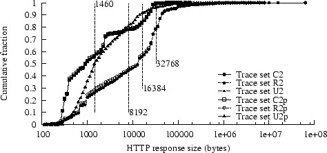 |
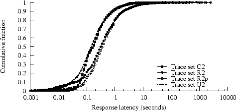
Figure 3:
CDF of status-200 response latencies
 |
The mean values in Table 1
do not convey the whole story. In
Figures 2
and 3, respectively,
we plot
cumulative distributions for
response size and latency for status-200 responses
(These plots exclude the U3 and U4 traces, since these CDFs
are nearly identical to those for the U2 trace;
Figure 3 also excludes C2p and U2p, since these CDFs
are nearly identical to those for the unpruned traces.)
The three traces in
Figure 2 show quite different response size distributions.
The responses in trace C2 seem somewhat smaller than has typically
been reported for Web traces; the responses in trace R2 are
a lot larger. (These differences also appear in the mean
response sizes in Table 1.)
Trace R2 is unusual, in part, because many users of
the site download entire technical reports, which tend to be
much larger than individual HTML or embedded-image files.
Figure 2 includes three vertical lines indicating
the 8K byte, 16K byte, and 32K byte thresholds. Note that 8K is
below the median size for R2, but above the median size for C2 and U2,
but the median for all traces is well below 32K bytes.
Figure 3 shows that response durations are significantly
longer in the R2 trace than in the others, possibly because of
the longer response sizes in R2.
Figure 4:
PDF of mean bandwidth per client
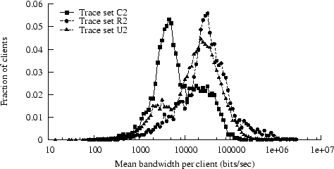 |
We calculated, for each distinct client, a mean bandwidth across
all transfers for that client.
Figure 4 shows the distributions; the pruned
traces had similar distributions and are not shown. Trace C2
has a much larger fraction of low-bandwidth users than R2 or U2.
The apparent slight excess of high-bandwidth clients in R2 might
result from the larger responses in R2; larger transfers generally
increase TCP's efficiency at using available bandwidth.
We also looked at the distribution of the TCP Maximum Segment
Size (MSS) values in our traces.
In trace R2, virtually all of the MSS values were at or close to the
standard Ethernet limit (about 1460 bytes); in traces C2 and U2,
about 95% of the MSS values were near the limit, with the rest
mostly close to 512 bytes.
Figure 2 shows a vertical line at 1460 bytes,
indicating approximately where the dominant MSS value lies on the
response-size distribution.
3.5 Trace anomalies
The monitoring architectures available to us differed at
each of the collection sites. For example, at one of the
sites port mirroring was used to copy packets from a
monitored link to the mirrored link. At
another site, separate links were tapped, one for
packets bound for the Web server, the second for packets sent
by the server. These monitoring infrastructures are subject
to a variety of measurement errors:
- Port mirroring multiplexes bidirectional traffic
from the monitored link onto the unidirectional mirror link.
This can cause packets to appear in the trace in a different
order than they arrived on the monitored link. Such reordering
typically affects packets that occurred close together in time.
For example, in the U2 trace, 10% of connections had
the SYN and SYNACK packets in reverse order. Our
Bro script corrects for this.
- Port mirroring temporarily buffers packets from the
monitored link until they can be sent over the mirrored link.
This buffer can overflow, causing
packets to be dropped.
- Several of our environments have multiple network
links that transfer packets to or from the Web server. Since we
could not monitor all of these links, we did not capture all of
the HTTP request/response transactions.
In some cases we capture
only half of the transaction (about 48% of the connections are affected
by this in one trace).
- Ideally, a traced packet would be timestamped at the precise instant it
arrives. However,
trace-collection systems buffer packets at least
briefly (often in several places) before attaching a timestamp,
and packets are often collected at several nearby points (e.g.,
two packet monitors on both members of a pair of simplex links),
which introduces timestamp errors due to imperfect clock synchronization.
Erroneous timestamps could cause errors in our analysis by affecting either
or both of our RTT estimates and our latency estimates.
Table 2:
Packet loss rates
| |
Total |
Total |
Measurement |
Retransmitted |
Conns. w/ |
Conns. w/no pkts |
| Trace name |
packets |
Conns. |
system lost pkts. |
packets |
retransmitted packets |
in one direction |
| C2 |
40474900 |
1182499 |
17017 (0.04%) |
114911 (0.3%) |
53906 (4.6%) |
572052 (48.4%) |
| R2 |
2824548 |
43023 |
1238 (0.04%) |
27140 (1.0%) |
4478 (10.4%) |
460 (1.1%) |
| U2 |
11335406 |
313462 |
5611 (0.05%) |
104318 (0.9%) |
26815 (8.6%) |
17107 (5.5%) |
| U3 |
11924978 |
328038 |
2093 (0.02%) |
89178 (0.7%) |
26371 (8.0%) |
14975 (4.6%) |
| U4 |
14393790 |
384558 |
5265 (0.04%) |
110541 (0.8%) |
30638 (8.0%) |
18602 (4.8%) |
|
|
|
|
|
|
|
|
We estimated the number of packets lost within our measurement system
by watching for gaps in the TCP sequence numbers. This could
overestimate losses (e.g., due to reordered packets) but
the estimates, as reported in Table 2, are quite low.
Table 2 also shows our estimates (based on a separate
Bro script) for
packet retransmission rates on the path between client
and server, implied by packets that cover part of the TCP sequence
space we have already seen. Retransmissions normally reflect packet
losses in the Internet, which would invalidate the model
used in equation 1. Knowing these rates could help understand
where the initial-RTT approach is applicable.
Note that Table 1 only includes connections with at least one
complete HTTP response, while Table 2 includes all connections,
including those that end in errors.
We were only able to use 27% of the connections listed
in Table 2 for C2, partly because we only saw
packets in one direction for 48% of the connections.
Our analysis script
flagged another  20% of the C2 connections
as error_has_occurred, possibly
due to unknown problems in the monitoring infrastructure. 20% of the C2 connections
as error_has_occurred, possibly
due to unknown problems in the monitoring infrastructure.
4 Predictions based on initial RTT: results
In this section, we summarize the results of our experiments
on techniques to predict transfer latency using the initial
RTT. We address these questions:
- Does RTT per se correlate well with latency?
- How well does equation 1 predict latency?
- Can we improve on equation 1?
- What is the effect of modem compression?
- How sensitive are the predictions to parameter choices?
There is no single way to define what it means for a latency
predictor to provide ``good'' predictions. We evaluate prediction
methods using several criteria, including the correlation between predicted
and measured latencies, and the mean and median of the difference
between the actual and predicted latencies.
4.1 Does RTT itself correlate with latency?
Figure 5:
Scatter plot of bandwidth vs. RTT, trace C2
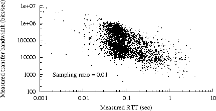 |
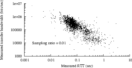
Figure 6:
BW vs. RTT, trace C2, 1 MSS  length 32KB length 32KB
 |
Perhaps it is unnecessary to invoke the full complexity of
equation 1 to predict latency from RTT.
To investigate this, we examined the correlation between
RTT per se and either bandwidth or latency.
For example,
Figure 5 shows a scatter plot of bandwidth vs. initial RTT,
for all status-200 responses in trace
C2.
(In order to avoid oversaturating our scatter plots,
we randomly sampled the actual data in each plot; the sampling
ratios are shown in the figures.)
The graph shows an apparent weak correlation between initial RTT
and transfer bandwidth.
Corresponding scatter plots for R2, U2, U3, and U4 show even
weaker correlations.
We found a stronger correlation
if we focused on transfer lengths above one MSS and
below 32K bytes,
as shown in Figure 6.
Our technique for measuring latency is probably least accurate
for responses below one MSS (i.e., those sent in just one packet).
Also,
single-packet responses may suffer excess apparent delay (as
measured by when the server receives the final ACK) because of
delayed acknowledgment at the client.
In our subsequent analyses, we exclude responses with lengths
of one MSS or less because of these measurement difficulties.
The 32KB threshold represents one plausible choice for defining
a ``short'' transfer.
Table 3:
Correlations: RTT vs. either bandwidth or latency
|
| Trace |
Samples |
Correlation |
Correlation |
| name |
included |
w/bandwidth |
w/latency |
| C2 |
140234 (24.3%) |
-0.352 |
0.511 |
| C2p |
129661 (24.3%) |
-0.370 |
0.508 |
| R2 |
7500 (18.7%) |
-0.112 |
0.364 |
| R2p |
5519 (17.6%) |
-0.054 |
0.418 |
| U2 |
218280 (37.6%) |
-0.163 |
0.448 |
| U2p |
181180 (37.8%) |
-0.178 |
0.458 |
| U3 |
234591 (36.8%) |
-0.181 |
0.421 |
| U3p |
181276 (36.9%) |
-0.228 |
0.427 |
| U4 |
283993 (37.2%) |
-0.179 |
0.364 |
| U4p |
219472 (37.3%) |
-0.233 |
0.411 |
(a) 1 MSS length 8KB
| Trace |
Samples |
Correlation |
Correlation |
| name |
included |
w/bandwidth |
w/latency |
| C2 |
261931 (45.4%) |
-0.325 |
0.426 |
| C2p |
238948 (44.8%) |
-0.339 |
0.426 |
| R2 |
20546 (51.4%) |
-0.154 |
0.348 |
| R2p |
15407 (49.0%) |
-0.080 |
0.340 |
| U2 |
312090 (53.7%) |
-0.165 |
0.392 |
| U2p |
258049 (53.8%) |
-0.179 |
0.401 |
| U3 |
336443 (52.8%) |
-0.162 |
0.263 |
| U3p |
259028 (52.7%) |
-0.215 |
0.276 |
| U4 |
414209 (54.2%) |
-0.167 |
0.287 |
| U4p |
320613 (54.4%) |
-0.215 |
0.343 |
(b) 1 MSS length 32KB
|
For a more quantified evaluation of this simplistic approach,
we did a statistical analysis using a simple R [18] program.
The
results are shown in Table 3(a) and (b), for lengths
limited to 8K and 32K bytes, respectively.
The tables show rows for both
pruned and unpruned versions of the five basic traces.
We included only status-200 responses whose length was at least
one MSS; the ``samples included'' column shows that count for each
trace.
The last two columns show the computed correlation between initial RTT
and either transfer bandwidth or transfer latency.
(The bandwidth correlations are negative, because this is
an inverse relationship.)
For the data set including response lengths up to 32K bytes,
none of these correlations exceeds 0.426, and many are much
lower.
If we limit the response lengths to 8K bytes, the correlations
improve, but this also eliminates most of the samples.
We tried excluding samples with an initial RTT value above
some quantile, on the theory that high RTTs correlate with
lossy network paths; this slightly improves RTT vs. bandwidth
correlations (for example, excluding records with an RTT above
281 msec reduces the number of 32K-or-shorter samples for R2 by 10%, and
improves that correlation from -0.154 to -0.302) but it actually worsens
the latency correlations (for the same example, from 0.348 to
0.214).
Note that, contrary to our expectation that traces pruned
of proxies and robots would be less predictable, in
Table 3 this seems
true only for the R2 trace; in general, pruning seems to
slightly improve predictability.
In fact, while we present results for both pruned and unpruned
traces throughout the paper, we see no consistent difference in
predictability.
4.2 Does equation 1 predict latency?
Although we did not expect RTT to correlate well with latency,
we might expect better results from the sophisticated model
derived by
Cardwell et al. [2]. They validated
their model (equation 1 is a simplified version)
using HTTP transfers over the Internet, but apparently used
only ``well-connected'' clients and so did not probe its utility
for poorly-connected clients. They also used RTT estimates that
included more samples than just each connection's initial RTT.
We therefore analyzed the ability of equation 1
to predict transfer bandwidths and latencies using only the
initial RTT, and with the belief that our traces include
some poorly-connected clients.
Figure 7:
Real vs. predicted latency, trace C2
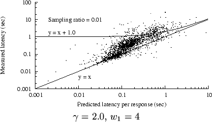 |
Figure 7 shows an example scatter plot of
measured latency vs. predicted latency, for trace C2. Again,
we include only status-200 responses at least one MSS in length.
We have superimposed two curves on the plot.
(Since this is a log-log plot, most linear equations result
in curved lines.)
Any point above
the line  represents an underprediction of latency;
underpredictions are generally worse than overpredictions, if (for
example) we want to avoid exposing Web users to unexpectedly long downloads.
Most of the points in the plot are above that line, but most
are below the curve represents an underprediction of latency;
underpredictions are generally worse than overpredictions, if (for
example) we want to avoid exposing Web users to unexpectedly long downloads.
Most of the points in the plot are above that line, but most
are below the curve
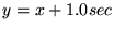 , implying that most of the
overpredictions (in this example) are less than 1 sec in excess.
However, a significant number are many seconds too high. , implying that most of the
overpredictions (in this example) are less than 1 sec in excess.
However, a significant number are many seconds too high.
We extended our R program to compute
statistics for the predictive ability of
equation 1. For each status-200 trace record with
a length between one MSS and 32K bytes,
we used the equation to predict a latency, and
then compared this to the latency recorded in the trace
record. We then computed the correlation between the actual
and predicted latencies.
We also computed a residual error value, as the difference
between the actual and predicted latencies.
Table 4 shows the results from this analysis,
using  and and  , a parameter assignment that
worked fairly well across all five traces. , a parameter assignment that
worked fairly well across all five traces.
Table 4:
Quality of predictions based on equation 1
|
| Trace |
Samples |
Correlation |
Median |
Mean |
| name |
included |
w/latency |
residual |
residual |
C2 |
261931 (45.4%) |
0.581 |
-0.017 |
0.164 |
| C2p |
238948 (44.8%) |
0.584 |
-0.015 |
0.176 |
| R2 |
20546 (51.4%) |
0.416 |
-0.058 |
0.261 |
| R2p |
15407 (49.0%) |
0.421 |
-0.078 |
0.272 |
| U2 |
312090 (53.7%) |
0.502 |
-0.022 |
0.110 |
| U2p |
258049 (53.8%) |
0.519 |
-0.024 |
0.124 |
| U3 |
336443 (52.8%) |
0.334 |
-0.018 |
0.152 |
| U3p |
259028 (52.7%) |
0.353 |
-0.016 |
0.156 |
| U4 |
414209 (54.2%) |
0.354 |
-0.013 |
0.141 |
| U4p |
320613 (54.4%) |
0.425 |
-0.010 |
0.136 |
Residual values are measured in seconds;
1 MSS length 32KB
|
In Table 4, the median residuals are always negative,
implying that equation 1 overestimates the transfer
latency more often than it underestimates it. However,
the mean residuals are always positive, because the equation's
underestimates are more wrong (in absolute terms) than its overestimates.
The samples in Figure 7 generally
follow a line with a steeper slope than , suggesting that
equation 1 especially underestimates higher
latencies.
One possible reason is that, for lower-bandwidth links, RTT
depends on packet size. For a typical 56Kb/s modem link, a SYN
packet will see an RTT somewhat above 100 msec, while a 1500 byte data
packet will see an RTT several times larger. This effect
could cause equation 1 to underestimate transfer
latencies.
4.3 Can we improve on equation 1?
Given that equation 1 seems to systematically
underestimate higher
latencies, exactly the error that we want to avoid, we realized
that we could modify the equation to reduce these errors.
We experimented with several modifications, including a linear
multiplier, but one simple approach is:
That is, we ``overpredict'' by a term proportional to the square
of the original prediction.
This is a heuristic, not the result of rigorous theory.
We found by trial and error that
a proportionality constant, or
``compensation weight,''
 worked best
for C2, but worked best
for C2, but
 worked
better for R2 U2, and worked
better for R2 U2, and
 worked best for U3 and U4.
For all traces, worked best for U3 and U4.
For all traces,  got the best results, and
we set got the best results, and
we set  for C2 and U2, and for C2 and U2, and  for R2, U3, and U4.
We discuss the sensitivity
to these parameters in Section 4.5. for R2, U3, and U4.
We discuss the sensitivity
to these parameters in Section 4.5.
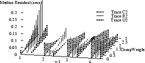
Figure 8:
Modified prediction results, trace C2
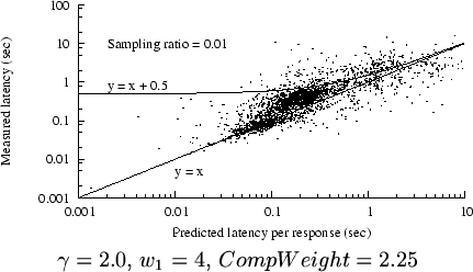 |
Figure 8 shows how the modified prediction
algorithm systematically overpredicts at higher latencies,
while not significantly changing the accuracy for lower latencies.
(For example, in this figure,
;
if equation 1 predicts a latency
of 0.100 seconds, the modified prediction will be 0.1225 seconds).
However, even the modified algorithm significantly underpredicts
a few samples; we do not believe we can avoid this, especially
for connections that suffer packet loss (see Table 2).
Table 5:
Predictions based on modified equation 1
| Trace |
Samples |
Correlation |
Median |
Mean |
| name |
included |
w/latency |
residual |
residual |
C2 |
261931 (45.4%) |
0.417 |
0.086 |
-0.002 |
| C2p |
238948 (44.8%) |
0.423 |
0.092 |
-0.006 |
| R2 |
20546 (51.4%) |
0.278 |
0.015 |
0.002 |
| R2p |
15407 (49.0%) |
0.311 |
0.019 |
0.013 |
| U2 |
312090 (53.7%) |
0.386 |
0.053 |
0.010 |
| U2p |
258049 (53.8%) |
0.402 |
0.056 |
0.001 |
| U3 |
336443 (52.8%) |
0.271 |
0.034 |
0.011 |
| U3p |
259028 (52.7%) |
0.302 |
0.036 |
-0.020 |
| U4 |
414209 (54.2%) |
0.279 |
0.035 |
0.003 |
| U4p |
320613 (54.4%) |
0.337 |
0.038 |
-0.033 |
Residual values are measured in seconds;
1 MSS length 32KB
|
Table 5 shows that the modifications
to equation 1 generally worsen the correlations,
compared to those in Table 4, but definitely
improves the residuals - the median error is always
less than 100 msec,
and the mean error is less than 15 msec, except for
traces U3p and U4p (our parameter choices were tuned for
the unpruned traces).
4.4 Text content and modem compression
Many people still use dialup modems.
It has been observed that to accurately model path bandwidth,
one must account for the compression typically done by
modems [3].
However, most image Content-Types are already compressed, so
this correction should only be done for text content-types.
Table 6:
Counts and frequency of content-types (excluding some rarely-seen types)
| Content-type |
C2 |
R2 |
U2 |
U3 |
U4 |
| Unknown |
3 (0.00%) |
26 (0.06%) |
178 (0.03%) |
157 (0.02%) |
144 (0.02%) |
| TEXT/* |
122426 (21.22%) |
23139 (57.83%) |
85180 (14.67%) |
92108 (14.45%) |
107958 (14.14%) |
| IMAGE/* |
454458 (78.78%) |
13424 (33.55%) |
465160 (80.10%) |
507330 (79.60%) |
607520 (79.57%) |
| APPLICATION/* |
0 (0.00%) |
3410 (8.52%) |
29733 (5.12%) |
37581 (5.90%) |
47765 (6.26%) |
| VIDEO/* |
0 (0.00%) |
4 (0.01%) |
17 (0.00%) |
10 (0.00%) |
5 (0.00%) |
| AUDIO/* |
0 (0.00%) |
8 (0.02%) |
446 (0.08%) |
194 (0.03%) |
140 (0.02%) |
|
HTTP responses normally carry a MIME Content-Type label,
which allowed us to analyze trace subsets for ``text/*''
and ``image/*'' subsets.
Table 6 shows the distribution of these coarse
Content-Type distinctions for the traces.
We speculated that the latency-prediction model of
equation 1, which incorporates
the response length, could be further improved by reducing
this length value when compression might be expected.
(A server making predictions knows the Content-Types of
the responses it plans to send.
Some servers might use a compressed content-coding for text
responses, which would obviate the need to correct predictions
for those responses for modem compression. We found no such
responses in our traces.)
We cannot directly predict either the compression ratio
(which varies among responses and among modems) nor can we
reliably determine which clients in our traces used modems.
Therefore, for feasibility of analysis
our model assumes a constant compressibility
factor for text responses, and we tested several plausible
values for this factor. Also, we assumed that an RTT
below 100 msec implied a non-modem connection, and RTTs
above 100 msec implied the possible use of a modem.
In a real system, information
derived from the client address might identify
modem-users more reliably.
(In Section 5 we classify clients using hostnames;
but this might add too much DNS-lookup delay to be effective
for latency prediction.)
Table 7:
Predictions for text content-types only
| Trace |
Samples |
Correlation |
Median |
Mean |
| name |
included |
w/latency |
residual |
residual |
C2 |
118217 (96.6%) |
0.442 |
0.142 |
0.002 |
| C2p |
106120 (96.4%) |
0.449 |
0.152 |
-0.003 |
| R2 |
12558 (54.3%) |
0.288 |
0.010 |
0.066 |
| R2p |
8760 (50.2%) |
0.353 |
0.017 |
0.105 |
| U2 |
70924 (83.3%) |
0.292 |
0.100 |
0.073 |
| U2p |
56661 (83.0%) |
0.302 |
0.110 |
0.066 |
| U3 |
76714 (83.3%) |
0.207 |
0.063 |
-0.021 |
| U3p |
56070 (83.2%) |
0.198 |
0.072 |
-0.099 |
| U4 |
90416 (83.8%) |
0.281 |
0.065 |
-0.034 |
| U4p |
65708 (83.8%) |
0.359 |
0.078 |
-0.122 |
Residual values are measured in seconds;
1 MSS length 32KB
|
Table 7 shows results for text
content-types only, using the modified prediction algorithm
based on equation 1, but without correcting
for possible modem compression.
We set  for C2 and U2, and
for R2, U3, and U4; for C2 and U2, and
for R2, U3, and U4;
 for C2 and for the other traces;
and for C2 and for the other traces;
and
 for all traces.
(We have not tested a wide range of for all traces.
(We have not tested a wide range of  values
to see if text content-types would benefit from a different
.)
Compared to the results for all
content types (see Table 5), the residuals
for text-only samples are generally higher. values
to see if text content-types would benefit from a different
.)
Compared to the results for all
content types (see Table 5), the residuals
for text-only samples are generally higher.
Table 8:
Predictions for text with compression
| Trace |
Samples |
Compression |
Correlation |
Median |
Mean |
| name |
included |
factor |
w/latency |
residual |
residual |
C2 |
118217 |
1.0 |
0.442 |
0.142 |
0.002 |
| C2p |
106120 |
1.0 |
0.449 |
0.152 |
-0.003 |
| R2 |
12558 |
4.0 |
0.281 |
0.013 |
0.002 |
| R2p |
8760 |
4.0 |
0.345 |
0.021 |
0.044 |
| U2 |
70924 |
3.0 |
0.295 |
0.083 |
0.008 |
| U2p |
56661 |
3.0 |
0.306 |
0.096 |
-0.004 |
| U3 |
76714 |
4.0 |
0.208 |
-0.002 |
0.001 |
| U3p |
56070 |
4.0 |
0.201 |
0.003 |
-0.063 |
| U4 |
90416 |
4.0 |
0.277 |
-0.000 |
-0.011 |
| U4p |
65708 |
4.0 |
0.353 |
0.007 |
-0.083 |
Residual values are measured in seconds;
1 MSS length 32KB
|
Table 8 shows results for text content-types
when we assumed that modems compress these by the factor shown
in the third column.
Note that for C2 and C2p, we got the best results using
a compression factor of 1.0 - that is, without correcting
for compression.
For the other traces, correcting for compression did give
better results.
Here we set the other parameters as:
(except for U3 and U4, where
worked best),
(except for C2, where worked best),
and
 (except for R2, where
worked best).
We experimented with assuming that the path did not involve
a modem (and thus should not be corrected for compression)
if the initial RTT was under 100 msec, but for R2 and U2
it turned out that we got the best results when we assumed
that all text responses should be corrected for compression. (except for R2, where
worked best).
We experimented with assuming that the path did not involve
a modem (and thus should not be corrected for compression)
if the initial RTT was under 100 msec, but for R2 and U2
it turned out that we got the best results when we assumed
that all text responses should be corrected for compression.
Table 8 shows that, except for trace C2,
correcting for modem compression improves
the mean residuals over those in Table 7.
We have not evaluated the use of compression factors
other than integers between 1 and 4, and
we did not evaluate a full range of values
for this section.
4.4.0.1 Image content
As shown in Table 6, image content-types dominate
most of the traces, except for R2. Also, Web site designers
are more likely to have choices between rich and simple
content for image types than for text types. (Designers
often include optional ``Flash'' animations, but we found
almost no Flash content in C2 and R2, and relatively little
in U2, U3, and U4.)
We therefore compared the predictability of transfer latencies
for image content-types, but found no clear difference
compared to the results for all content in general.
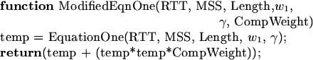
4.5 Sensitivity to parameters
How sensitive is prediction performance to the parameters
 , ,  , and ? That
question can be framed in several ways: how do the results
for one server vary with parameter values? If parameters
are chosen based on traces from server X, do they work well
for server Y? Are the optimal values constant over time,
client sub-population,
content-type, or response length? Do optimal parameter
values depend on the performance metric?
For reasons of space, we focus on the first two of these questions. , and ? That
question can be framed in several ways: how do the results
for one server vary with parameter values? If parameters
are chosen based on traces from server X, do they work well
for server Y? Are the optimal values constant over time,
client sub-population,
content-type, or response length? Do optimal parameter
values depend on the performance metric?
For reasons of space, we focus on the first two of these questions.
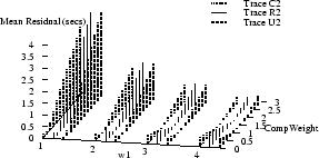
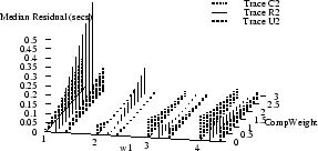
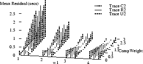
Figure 9 shows how the absolute values of
the mean and median
residuals vary with , , and for
traces C2, R2, and U2.
The optimal parameter choice depends on whether
one wants to minimize the mean or the median; for example,
for R2,
, , and
yields
an optimal mean of 1.5 msec (and a median of 15 msec). The
median can be further reduced to 0.2 msec, but at the cost
of increasing the mean to over half a second.
Figure 9 also shows how the optimal parameters
vary across several traces.
(Results for traces U3 and U4 are similar to those for U2,
and are omitted to reduce clutter.)
It appears that no single choice
is optimal across all traces, although some choices
yield
relatively small mean and medians for many traces.
For example, , , and
yields optimal or near-optimal mean residuals for U2,
U3, and U4, and decent results for C2.
4.6 Training and testing on different data
The results we have presented so far used parameter
choices ``trained'' on the same data sets as our results
were tested on. Since any real prediction system requires
advance training, we also evaluated predictions with
training and testing on different data sets.
Our trace collection was not carefully designed in this
regard; we have no pairs of data sets that are completely
identical and adjacent in time. For the C2, R2, and U2
data sets, we chose the first three days as the
training data set, and the last four days as the testing
data set. However, because we collected data at different
hours on each day, and because there are day-of-week differences
between the training and testing sets (the testing
sets includes two weekend days), we suspect that these
pairs of data sets might not be sufficiently similar.
We also used the U3 data set to train parameters that
we then tested on the U4 data set; these two traces are
more similar to each other.
Table 9:
Training and testing on different data
|
| |
Trained parameters |
|
Testing results |
| |
|
|
|
residual |
rank |
|
|
| Trace |
|
|
Comp |
in |
(of |
|
best |
| name |
|
|
Weight |
training |
96) |
residual |
resid. |
C2 |
2.0 |
4 |
2.50 |
-0.000 |
15 |
-0.098 |
-0.004 |
| C2p |
2.0 |
3 |
1.75 |
-0.004 |
12 |
-0.089 |
-0.002 |
| R2 |
1.5 |
4 |
1.50 |
-0.004 |
20 |
0.136 |
0.000 |
| R2p |
1.5 |
3 |
1.00 |
0.003 |
16 |
0.125 |
0.003 |
| U2 |
1.5 |
4 |
1.50 |
0.001 |
10 |
-0.072 |
0.012 |
| U2p |
2.0 |
2 |
0.75 |
-0.004 |
9 |
-0.081 |
-0.002 |
| U3U4 |
2.0 |
2 |
0.75 |
-0.007 |
3 |
-0.013 |
0.003 |
| U3U4p |
2.0 |
1 |
0.25 |
0.000 |
2 |
-0.013 |
-0.010 |
Residual values are measured in seconds;
1 MSS length 32KB
|
Table 9 shows results for training vs. testing.
We tested and trained with
96 parameter combinations, based on
the two possible choices for , the four choices for ,
and twelve equally-spaced choices for .
The trained parameters are those that minimize the absolute
value of the mean residual in training.
The columns under testing results show how the results
using the trained parameters rank among all of the testing results,
the mean residual when using those parameters, and the residual
for the best possible parameter combination for the testing data.
These results suggest that the degree to which training
can successfully select parameter values might vary
significantly from site to site. Based on our traces,
we would have had the most success making useful predictions
at the University site (U3-U4), and the least success at the Research site
(R2).
However, the difference in ``trainability'' that we observed
might instead be the result of the much closer match between
the U3 and U4 datasets, compared to the time-of-day and
day-of-week discrepancies in the other train/test comparisons.
For C2, R2, and U2, we tried training just on one day
(Tue., May 4, 2004) and testing on the next day, and got
significantly better trainability (except for R2p, which was
slightly worse) than in Table 9; this supports
the need to match training and testing data sets more carefully.
4.7 A server's decision algorithm
To understand how a server might use the initial-RTT approach in
practice, Figure 10 presents pseudo-code for generating
predictions.
(This example is in the context of a Web server adapting its
content based on predicted transfer latency, but the basic
idea should apply to other contexts.)
If the server has  choices of response length
for a given request, it would invoke PredictLatency choices of response length
for a given request, it would invoke PredictLatency  times, starting with the largest
candidate and moving down in size, until it either finds one with a
small-enough predicted latency, or has only one choice left.
The first three arguments to the PredictLatency
function (RTT, MSS, and client IP address) are known as soon as the
connection is open. The last two (response content type and length)
are specific to a candidate response that the server might send.
times, starting with the largest
candidate and moving down in size, until it either finds one with a
small-enough predicted latency, or has only one choice left.
The first three arguments to the PredictLatency
function (RTT, MSS, and client IP address) are known as soon as the
connection is open. The last two (response content type and length)
are specific to a candidate response that the server might send.
Figure 10:
Pseudo-code for the decision algorithm
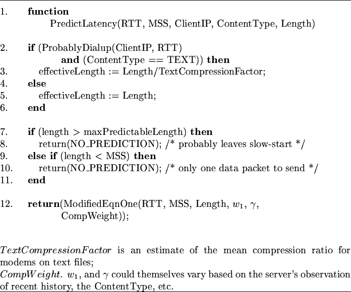 |
The function ProbablyDialup, not shown here, is a heuristic
to guess whether a client is connected via a modem (which would
probably compress text responses). It could simply assume that
RTTs above 100 msec are from dialups, or it could use additional
information based on the client's DNS name or AS (Autonomous System)
number to identify likely dialups.
5 Detecting dialups
We speculated that a server could discriminate between dialups
and non-dialups using clues from the client's ``fully-qualified
domain name'' (FQDN). We obtained FQDNs for about 75% of the
clients in the U4 trace, and then grouped them according to clues
in the FQDNs that implied geography and network technology.
Note that many could not be categorized by this method, and
some categorizations are certainly wrong.
Table 10:
RTTs by geography and connection type
| Category |
Conns. |
5%ile |
median |
mean |
95%ile |
| By geography |
| All |
326359 |
0.008 |
0.069 |
0.172 |
0.680 |
| N. America |
35972 |
0.003 |
0.068 |
0.124 |
0.436 |
| S. America |
2372 |
0.153 |
0.229 |
0.339 |
0.882 |
| Europe |
12019 |
0.131 |
0.169 |
0.262 |
0.717 |
| Asia-Pacific |
9176 |
0.165 |
0.267 |
0.373 |
0.885 |
| Africa |
2027 |
0.206 |
0.370 |
0.486 |
1.312 |
| "Dialup" in FQDN |
| All |
11478 |
0.144 |
0.350 |
0.664 |
2.275 |
| Regional |
5977 |
0.133 |
0.336 |
0.697 |
2.477 |
| Canada |
1205 |
0.208 |
0.460 |
0.751 |
2.060 |
| US |
575 |
0.189 |
0.366 |
0.700 |
2.210 |
| Europe |
566 |
0.183 |
0.216 |
0.313 |
0.861 |
| "DSL" in FQDN |
| All |
59211 |
0.003 |
0.023 |
0.060 |
0.210 |
| Local |
1816 |
0.011 |
0.022 |
0.034 |
0.085 |
| Regional |
47600 |
0.009 |
0.018 |
0.032 |
0.079 |
| US |
1053 |
0.071 |
0.085 |
0.117 |
0.249 |
| Europe |
118 |
0.148 |
0.162 |
0.178 |
0.313 |
| "Cable" in FQDN |
| All |
6599 |
0.039 |
0.077 |
0.132 |
0.338 |
| Canada |
2741 |
0.039 |
0.055 |
0.088 |
0.222 |
| US |
585 |
0.072 |
0.086 |
0.094 |
0.127 |
| Europe |
600 |
0.143 |
0.155 |
0.176 |
0.244 |
Times in seconds; bold entries are  sec.
|
Table 10 shows how initial RTTs vary by
geography and connection type. For the connections that we
could categorize, at least 95% of ``dialup'' connections have
RTTs above 100 msec, and most ``cable'' and
``DSL'' connections have RTTs below 200 msec.
These results seem unaffected by further geographical
subdivision, and support the hypothesis that a threshold
RTT between 100 and 200 msec would discriminate fairly
well between dialup and non-dialup connections. We do
not know if these results apply to other traces.
6 Predictions from previous bandwidths: results
In this section, we compare how well prediction based on
variants of equation 1 compares with predictions from
the older recent-transfers approach. We address these questions:
- How well can we predict latency from previous bandwidth
measurements?
- Does a combination of the two approaches improve on either
individual predictor?
Note that the recent-transfers approach cannot specifically
predict the latency for the very first transfer to a given
client, because the server has no history for that client.
This is a problem if the goal is to provide the best user
experience for a client's initial contact with a Web site.
For initial contacts, a server using the recent-transfers approach
to predict latency has several options, including:
- Make no prediction.
- ``Predict'' the latency based on history across all previous
clients; for example, use an exponentially smoothed mean of all previous
transfer bandwidths.
- Assume that clients with similar network locations, based on
routing information, have similar bandwidths; if a new client
belongs to ``cluster'' of clients with known bandwidths, use history
from that cluster to make a prediction. Krishnamurthy and
Wang [8] describe
a technique to discover clusters of client IP addresses.
Krishnamurthy and Wills [9]
then showed, using a set of chosen Web pages with various
characteristics, that clustering pays off in prediction
accuracy improvements ranging up to about 50%.
We speculate that this approach would also work for our traces.
- Use the initial-RTT technique to predict a client's first-contact
latency, and use the recent-transfers technique to predict
subsequent latencies for each client. We call this the
hybrid technique.
We first analyze the purest form of recent-transfers (making no
prediction for first-contact clients), and then consider the
mean-of-all-clients and hybrid techniques.
6.1 Does previous bandwidth predict latency?
Table 11:
Correlations: measured vs. recent bandwidths
| |
Correlation with |
| |
|
most |
mean |
weighted |
| Trace |
Samples |
recent |
previous |
mean |
| name |
included |
bandwidth |
bandwidth |
bandwidth |
| C2 |
262165 (45.4%) |
0.674 |
0.742 |
0.752 |
| C2p |
238957 (44.8%) |
0.658 |
0.732 |
0.737 |
| R2 |
24163 (60.4%) |
0.589 |
0.655 |
0.666 |
| R2p |
17741 (56.5%) |
0.522 |
0.543 |
0.579 |
| U2 |
310496 (53.5%) |
0.527 |
0.651 |
0.654 |
| U2p |
254024 (52.9%) |
0.437 |
0.593 |
0.561 |
| U3 |
341968 (53.7%) |
0.495 |
0.627 |
0.638 |
| U3p |
260470 (53.0%) |
0.508 |
0.659 |
0.625 |
| U4 |
421867 (55.3%) |
0.521 |
0.690 |
0.647 |
| U4p |
323811 (55.0%) |
0.551 |
0.690 |
0.656 |
Best correlation for each trace shown in bold
|
We did a statistical analysis of the prediction ability of
several variants of the pure recent-tranfers technique.
In each case, we made predictions and maintained history
only for transfer lengths of at least one MSS.
Table 11 shows the results.
The first two columns show the trace name
and the number of samples actually used in the analysis.
The next three columns show the correlations between the
bandwidth (not latency) in a trace record and, respectively, the most
recent bandwidth for the same client, the mean of previous
bandwidths for the client, and the exponential weighted mean
 .
We followed Krishnamurthy et al. [10]
in using .
We followed Krishnamurthy et al. [10]
in using  , although other values might work
better for specific traces. , although other values might work
better for specific traces.
These results suggest that some form of mean is the best
variant for this prediction technique; although the choice
between simple means and weighted means varies between traces,
these always outperform predictions based on just the most previous
transfer. Since Krishnamurthy et al. [10]
preferred the weighted mean, we follow their lead for the
rest of this paper.
Pruning the traces, as we had expected, does seem to decrease
the predictability of bandwidth values, except for the U3 and
U4 traces. This effect might
be magnified for the recent-transfers technique, since (unlike
the initial-RTT technique) it relies especially on intra-client
predictability.
Table 12:
Latency prediction via weighted mean bandwidth
|
| Trace |
Samples |
Correlation |
Median |
Mean |
| name |
included |
w/latency |
residual |
residual |
C2 |
262165 (45.4%) |
0.514 |
-0.042 |
-0.502 |
| C2p |
238957 (44.8%) |
0.515 |
-0.046 |
-0.529 |
| R2 |
24163 (60.4%) |
0.525 |
-0.066 |
-4.100 |
| R2p |
17741 (56.5%) |
0.560 |
-0.140 |
-5.213 |
| U2 |
310496 (53.5%) |
0.475 |
-0.028 |
-1.037 |
| U2p |
254024 (52.9%) |
0.460 |
-0.033 |
-1.142 |
| U3 |
341968 (53.7%) |
0.330 |
-0.025 |
-1.138 |
| U3p |
260470 (53.0%) |
0.374 |
-0.029 |
-1.288 |
| U4 |
421867 (55.3%) |
0.222 |
-0.021 |
-0.957 |
| U4p |
323811 (55.0%) |
0.251 |
-0.024 |
-1.111 |
(a) 1 MSS length
| Trace |
Samples |
Correlation |
Median |
Mean |
| name |
included |
w/latency |
residual |
residual |
C2 |
256943 (44.5%) |
0.516 |
-0.038 |
-0.485 |
| C2p |
234160 (43.9%) |
0.516 |
-0.043 |
-0.512 |
| R2 |
17445 (43.6%) |
0.317 |
-0.018 |
-0.779 |
| R2p |
12741 (40.6%) |
0.272 |
-0.054 |
-0.959 |
| U2 |
287709 (49.5%) |
0.256 |
-0.020 |
-0.407 |
| U2p |
235481 (49.1%) |
0.247 |
-0.024 |
-0.454 |
| U3 |
314965 (49.4%) |
0.447 |
-0.017 |
-0.300 |
| U3p |
239843 (48.8%) |
0.484 |
-0.020 |
-0.336 |
| U4 |
390981 (51.2%) |
0.338 |
-0.015 |
-0.274 |
| U4p |
299905 (50.9%) |
0.312 |
-0.017 |
-0.314 |
(a) 1 MSS length 32KB
|
Table 11 showed correlations between bandwidth
measurements and predictions. To predict a response's latency, one can
combine a bandwidth prediction with the known response length.
Table 12 shows how well the weighted mean bandwidth
technique predicts latencies.
Table 12(a) includes responses with length at
least one MSS; Table 12(b) excludes responses
longer than 32 Kbytes. Because short responses and long responses
may be limited by different parameters (RTT and bottleneck bandwidth,
respectively), we hypothesized that
it might not make sense to predict short-response
latencies based on long-response history.
Indeed, the residuals in Table 12(b) are
always better than the corresponding values in
Table 12(a), although the correlations are
not always improved.
The correlations in Table 12(a)
are better than those from the modified equation 1
as shown in Table 5, except for trace U4.
However, the mean residuals in Table 12 are much larger
in magnitude
than in Table 5; it might be possible to
correct the bandwidth-based predictor to fix this.
The previous-bandwidth approach consistently overpredicts latency, which in some
applications might be
better than underprediction. Figure 11 shows
an example scatter plot, for R2. In the Web-server content
adaptation application, excessive overprediction
increases the chances that a well-connected user will fail to
receive rich content, although this is less harmful than sending
excessive content to a poorly-connected user.
Figure 11:
Real vs. bandwidth-predicted latency, trace R2
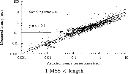 |
6.2 Combining predictors
Given that the initial-RTT approach seems more accurate at
predicting first-contact latencies, for many thresholds, than
the recent-transfers approach, we speculated that a hybrid
of the two predictors might yield the best results. This
hybrid would use the modified equation 1
predictor for a client's first-contact transfer, and the
smoothed mean of the client's previous bandwidths for its
subsequent transfers.
We found that the overall (all-transfers)
accuracy of this hybrid is nearly indistinguishable from the
overall accuracy of the recent-transfers approach because, as
the statistics in Table 1 imply, only a small fraction of
transfers in our traces are first contacts.
7 Summary and conclusions
We conducted a study, based on traces from
several different user communities, to demonstrate how well
two different approaches can predict the latency of short
TCP transfers. We found that by making a minor modification
to a previously-described formula, we could greatly reduce its
absolute prediction errors. We showed that predictions
based on observation of past history generally yield better
overall correlations than our formula-based predictor, but
the formula-based predictor has lower mean prediction errors.
We also show that the formula-based predictor could be improved
to handle the specific case of text content, where modem-based
compression can affect latency. Finally, we reported results from
a study on the relationship between round-trip time
and the use of modems, suggesting that this relationship might
be exploited to improve prediction accuracy.
This paper has not quantified how much a real application,
such as a Web server, could improve end-to-end performance
by using our prediction techniques. Our technical
report [1]
provides some additional analysis of this and other details
that do not fit here.
We would like to thank Vern Paxson, for his help with Bro
and especially for writing the first draft of our Bro script
and for improving Bro to meet our needs;
Jerry Shan, for lots of help with statistical analysis;
and
Mike Rodriquez, Oliver Spatscheck, and others
for their help in support of data collection.
We thank
Rick Jones,
Zhuoqing Morley Mao,
Dejan Milojicic,
Mehul Shah,
Chris Tuttle,
Carey Williamson,
and the anonymous reviewers
for their helpful comments.
- 1
-
ARLITT, M., KRISHNAMURTHY, B., AND MOGUL, J. C.
Predicting short-transfer latency from TCP arcana: extended
version.
Tech. Report HPL-2005-137, HP Labs, Sep 2005.
- 2
-
CARDWELL, N., SAVAGE, S., AND ANDERSON, T.
Modeling TCP latency.
In Proc INFOCOM (3) (Tel Aviv, Mar. 2000), pp. 1742-1751.
- 3
-
CHENG, Y.-C., HÖLZLE, U., CARDWELL, N., SAVAGE, S., AND VOELKER,
G. M.
Monkey See, Monkey Do: A Tool for TCP Tracing and Replaying.
In Proc. USENIX Annual Tech. Conf. (Boston, MA, June 2004),
pp. 87-98.
- 4
-
CHESHIRE, S.
Latency and the quest for interactivity, Nov. 1996.
https://www.stuartcheshire.org/papers/LatencyQuest.ps.
- 5
-
CHESHIRE, S.
Latency survey results (for ``It's the Latency, Stupid'').
https://www.stuartcheshire.org/rants/LatencyResults.html, 1996.
- 6
-
FIELDING, R., GETTYS, J., MOGUL, J., FRYSTYK, H., MASINTER, L., LEACH, P.,
AND BERNERS-LEE, T.
RFC 2616: Hypertext transfer protocol--HTTP/1.1, June 1999.
- 7
-
HE, Q., DOVROLIS, C., AND AMMAR, M.
On the Predictability of Large Transfer TCP Throughput.
In Proc. SIGCOMM (Philadelphia, PA, Aug 2005).
- 8
-
KRISHNAMURTHY, B., AND WANG, J.
On network-aware clustering of Web clients.
In SIGCOMM (Stockholm, Aug. 2000), pp. 97-110.
- 9
-
KRISHNAMURTHY, B., AND WILLS, C. E.
Improving Web performance by client characterization driven server
adaptation.
In Proc. WWW2002 (Honolulu, HI, May 2002), pp. 305-316.
- 10
-
KRISHNAMURTHY, B., WILLS, C. E., ZHANG, Y., AND VISHWANATH, K.
Design, implementation, and evaluation of a client characterization
driven web server.
In Proc. WWW2003 (Budapest, May 2003), pp. 138-147.
- 11
-
LAI, K., AND BAKER, M.
Nettimer: A tool for measuring bottleneck link bandwidth.
In Proc. USITS (San Francisco, CA, Mar 2001), pp. 123-134.
- 12
-
MICROSOFT CORP.
Knowledge Base Article 254337: Internet Explorer Sends Two GET
Requests for the Same Data When the MIME Handler Is an ActiveX Control,
2000.
https://support.microsoft.com/default.aspx?scid=kb;en-us;254337.
- 13
-
MICROSOFT CORP.
Exchange 2003 Design and Architecture at Microsoft.
https://www.microsoft.com/technet/itsolutions/msit/deploy/ex03atwp.mspx, Aug 2003.
- 14
-
MICROSOFT CORP.
Knowledge Base Article 293792: Three GET Requests Are Sent When You
Retrieve Plug-in Served Content, 2003.
https://support.microsoft.com/default.aspx?scid=kb;en-us;293792.
- 15
-
MOGUL, J., AND BRAKMO, L.
Method for dynamically adjusting multimedia content of a web page by
a server in accordance to network path characteristics between client and
server.
U.S. Patent 6,243,761, June 2001.
- 16
-
MOGUL, J., BRAKMO, L., LOWELL, D. E., SUBHRAVETI, D., AND MOORE, J.
Unveiling the transport API.
In Proc. 2nd Workshop on Hot Topics in Networks (Cambridge,
MA, November 2003).
- 17
-
PAXSON, V.
Bro: A system for detecting network intruders in real-time.
Computer Networks 31, 23-24 (Dec. 1999), 2435-2463.
- 18
-
R DEVELOPMENT CORE TEAM.
R: A language and environment for statistical computing.
R Foundation for Statistical Computing, Vienna, Austria, 2003.
ISBN 3-900051-00-3.
- 19
-
SCHROEDER, B., AND HARCHOL-BALTER, M.
Web servers under overload: How scheduling can help.
ACM Trans. on Internet Techologies 6, 1 (Feb. 2006).
- 20
-
SU, J., CHIN, A., POPIVANOVA, A., GOEL, A., AND DE LARA, E.
User mobility for opportunistic ad-hoc networking.
In Proc. WMCSA (Lake District, UK, Dec 2004), pp. 41-50.
Predicting short-transfer latency from TCP arcana:
A trace-based validation
This document was generated using the
LaTeX2HTML translator Version 2002 (1.67)
Copyright © 1993, 1994, 1995, 1996,
Nikos Drakos,
Computer Based Learning Unit, University of Leeds.
Copyright © 1997, 1998, 1999,
Ross Moore,
Mathematics Department, Macquarie University, Sydney.
The command line arguments were:
latex2html -split 0 -no_navigation -no_footnode -show_section_numbers -numbered_footnotes -white imc05web.tex
The translation was initiated by Jeffrey Mogul on 2005-08-10
Jeffrey Mogul
2005-08-10
|