Designing Controllable Computer Systems

	Christos Karamanolis	Magnus Karlsson	Xiaoyun Zhu
	Hewlett-Packard Labs

Abstract:

1 Introduction

As the size and complexity of computer systems grow, system administration has become the predominant factor of ownership cost [6] and a main cause for reduced system dependability [14]. The research community has recognized the problem and there have been several calls to action [11,17]. All these approaches propose some form of self-managed, self-tuned systems that aim at minimizing manual administrative tasks.

As a result, computers are increasingly designed as closed-loop systems: as shown in Figure 1, a controller automatically adjusts certain parameters of the system, on the basis of feedback from the system. Examples of such closed-loop systems aim at managing the energy consumption of servers [4], automatically maximizing the utilization of data centers [16,18], or meeting performance goals in file servers [9], Internet services [10,12] and databases [13].

When applying dynamic control, it is important that the resulting closed-loop system is stable (does not exhibit large oscillations) and converges fast to the desired end state. Many existing closed-loop systems use ad-hoc controllers and are evaluated using experimental methods. We claim that a more rigorous approach is needed for designing dynamically controlled systems. In particular, we advocate the use of control theory, because it results in systems that can be shown to work beyond the narrow range of a particular experimental evaluation. Computer system designers can take advantage of decades of experience in the field and can apply well-understood and often automated methodologies for controller design.

Figure: A closed-loop system.

However, we believe that systems designers should not be concerned with the design of controllers. Control theory is an active research field on its own, which has produced streamlined control methods [2] or even off-the-shelf controller implementations [1] that systems designers can use. Indeed, we show that many computer management problems can be formulated so that standard controllers can be applied to solve them. Thus, the systems community should stick with systems design; in this case, systems that are amenable to dynamic, feedback-based control. That is, provide the necessary tunable system parameters (actuators) and export the appropriate feedback metrics (measurements), so that an off-the-shelf controller can be applied without destabilizing the system, while it ensures fast convergence to the desired goals. Traditionally, control theory has been concerned with systems that are governed by laws of physics (e.g., mechanical devices), thus allowing to make assertions about the existence or not of certain properties. This is not necessarily the case with software systems. We have seen in practice that checking whether a system is controllable or, even more, building controllable systems is a challenging task often involving non-intuitive analysis and system modifications.

As a first step in addressing the latter problem, this paper proposes a set of necessary and sufficient properties that any system must abide by to be controllable by a standard adaptive controller that needs little or no tuning for the specific system. These properties are derived from the theoretical foundations of a well-known family of adaptive controllers. The paper discusses the intuition and importance of these properties from a systems perspective and provides insights about the challenges facing the designer that tries to enforce them. The discussion has been motivated by lessons learned while designing self-managed systems for an adaptive enterprise environment [17]. In particular, we elaborate on the discussion of the properties with two very diverse management problems: 1) enforcing soft performance goals in networked service by dynamically adjusting the shares of competing workloads; 2) controlling the number of blades assigned to a workload to meet performance goals within power budgets.

2 Dynamic Control

Many computer management problems can be cast as on-line optimization problems. Informally speaking, the objective is to have a number of measurements obtained from the system converge to the desired goals by dynamically setting a number of system parameters (actuators). The problem is formalized as an objective function that has to be minimized. A formal problem specification is outside the scope of this paper. The key point here is that there are well-understood, standard controllers that can be used to solve such optimization problems. Existing research has shown that, in the general case, adaptive controllers are needed to trace the varying behavior of computer systems and their changing workloads [9,12,18].

2.1 Self-tuning regulators

For the discussion in this paper, we focus on one of the best-known families of adaptive controllers, namely Self-Tuning Regulators (STR)) [2], that have been widely used in practice to solve on-line optimization control problems. The term ``self-tuning'' comes from the fact that the controller parameters are automatically tuned to obtain the desired properties of the closed-loop system. The design of closed-loop systems involves many tasks such as modeling, design of control law, implementation, and validation. STR controllers aim at automating these tasks. Thus, they can be used out-of-the-box for many practical cases. Other types of adaptive controllers proposed in the literature usually require more intervention by the designer.

Figure: The components of a self-tuning regulator.

As shown in Figure 2, an STR consists of two basic modules: the model estimator module on-line estimates a model that describes the current measurements from the system as a function of a finite history of past actuator values and measurements; that model is then used by the control law module that sets the actuator values. We propose using a linear model of the following form for model estimation in the STR:

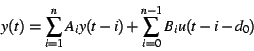(1)

Clearly, the relation between actuation and observed system behavior is not always linear. For example, while throughput is indeed a linear function of the share of resources (e.g., CPU cycles) assigned to a workload, the relation between latency and resource share is nonlinear as Little's law indicates. However, even in the case of nonlinear metrics, a linear model is often a good-enough local approximation to be used by a controller [2], as the latter usually only makes small changes to actuator settings. The advantage of using linear models is that they can be estimated in computationally efficient ways. Thus, they result in tractable control laws and they admit simpler analysis including stability proofs for the closed-loop system.

The control law is essentially a function that, based on the estimated system model (1) at time , decides what the actuator values should be to minimize the objective function. The STR derives from a closed-form expression as a function of previous actuations, previous measurements, model parameters and the reference values (goal) for the measurements. Details of the theory can be found in Åström et al.  [2]. From a systems perspective, the important point is that these are computationally efficient calculations that can be performed on-line. Moreover, an STR requires little system-specific tuning as it uses a dynamically estimated model of the system and the control law automatically adapts to system and workload dynamics.

2.2 Properties of controllable systems

For the aforementioned process to apply and for the resulting closed-loop system to be stable and to have predictable convergence time, control theory has derived a list of necessary and sufficient properties that the target system must abide by [2,7]. In the following paragraphs, we interpret these theoretical requirements into a set of system-centric properties. We provide guidelines about how one can verify whether a property is satisfied and what are the challenges for enforcing them.

C.1. Monotonicity. The elements of matrix in (1) must each have a known sign that remains the same over time.

The intuition behind this property is that the real (non estimated) relation between any actuator and any measurement must be monotonic and of known sign. This property usually refers to some physical law. Thus, it is generally easy to check for it and get the signs of . For example, in the long term, a process with a large share of CPU cycles gets higher throughput and lower latency than one with a smaller share.

C.2. Accurate models. The estimated model (1) is a good-enough local approximation of the system's behavior.

As discussed, the model estimation is performed periodically. A fundamental requirement is that the dynamic relation between actuators and measurements is captured sufficiently by the model around the current operating point of the system. In practice, this means that the estimated model must track only real system dynamics. We use the term noise to describe deviations in the system behavior that are not captured by the model. It has been shown that to ensure stability in linear systems where there is a known upper bound on the noise amplitude, the model should be updated only when the model error is twice the noise bound [5]. The theory is more complicated for non-linear systems [15], but the above principle can be used as a rule of thumb in that case too. There are a number of sources for the aforementioned noise:

1. System dynamics that have a frequency higher than that of sampling in the system, especially when one measures instantaneous values instead of averages over the sampling interval.
2. Sudden transient deviations from the operating range of the system. For example, rapid latency fluctuations because of contention on a shared network link.
3. A fundamentally volatile relation between certain actuators and measurements. One example is the relation between resource shares and provided throughput. When the aggregate throughput of the system oscillates a lot (as is often the case in practice), this relation is volatile. Instead, a more stable relation could be expressed as the fraction of the total system throughput received by a workload as a function of share.
4. Quantization errors when a linear model is used to approximate locally in an operating range the behavior of a nonlinear system.

In fact, a tiny actuation error has often to be introduced, so that the system is excited sufficiently for a good model to be derived. In other words, the system is forced to slightly deviate from its operating point to derive a linear model approximation (you need two points to draw a line). It is the controller that typically introduces such small perturbations for modeling purposes.

Picking actuators and measurement metrics that result in stable, ideally linear, relations is one of the most challenging and important tasks in the design of a controllable system, as we discuss in Section 3. The following two properties are also related to the requirement for accurate models.

C.3. Known system delay. There is a known upper bound on the time delay in the system.

C.4. Known system order. There is a known upper bound on the order of the system.

Property C.3 ensures that the controller knows when to expect the first effects of its actuations, while C.4 ensures that the model remembers sufficiently many prior measurements () and actuations () to capture the dynamics of the system. These properties are needed for the controller to be able to observe the effects of its actuations and then attempt to correct any error in subsequent actuations. If the model order was less than the actual system order, then the controller would not be aware of some of the causal relations between actuation and measurements in the system. The values of and are derived experimentally. The designer is faced with a trade-off: On one hand, the values of and must be sufficiently high to capture as much as possible of the causal relations between actuation and measurements. On the other hand, a high implies a slow-responding controller and a high increases the computational complexity of the STR. and are ideal values.

C.5. Minimum phase. Recent actuations have higher impact on the measurements than older actuations do.

A minimum phase system is basically one for which the effects of an actuation can be corrected or canceled by another, later actuation. It is possible to design STRs that deal with non-minimum phase systems, but they involve experimentation and non-standard design processes. In other words, without the minimum phase requirement, we cannot use off-the-shelf controllers. Typically, physical systems are minimum phase--the causal effects of events in the system fade as time passes by. Sometimes, however, this is not the case with computer systems, as we see in Section 3. To ensure this property, a designer must re-set any internal state that reflects older actuations. Alternatively, the sample interval can always be increased until the system becomes minimum phase. Consider, for example, a system where the effect of an actuation peaks after three sample periods. By increasing the sample period threefold, the peak is now contained in the first sample period, thus abiding by this property. Increasing the sample interval should only be a last resort, as longer sampling intervals result in slower control response.

C.6. Linear independence. The elements of each of the vectors and must be linearly independent.

Unless this property holds, the quality of the estimated model is poor: the predicted value for may deviate considerably from the actual measurements. The reason for this requirement is that some of the calculations in RLS involve matrix inversion. When C.6 is not satisfied, there exists a matrix internal to RLS that is singular or close to singular. When inverted, that matrix contains very large numbers, which in combination with the limited resolution of floating point arithmetic of a CPU, result in models that are wrong. Note that the property does not require that the elements in and in are completely non-correlated; they must not be linearly correlated. Often, simple intuition about a system may be sufficient to ascertain if there are linear dependencies among actuators, as we see in Section 3.

C.7. Zero-mean measurements and actuator values. The elements of each of the vectors and should have a mean value close to 0.

If the actuators or the measurements have a large constant component to them, RLS tries to accurately predict this constant component and may thus miss to capture the comparably small changes due to actuation. For example, when the measured latency (in ms) in a system varies in the range depending on the share of resources assigned to a workload, the model estimator would not accurately capture the relatively small changes due to the share actuation. If there is a large constant component in the measurements and it is known, then it can be simply deducted from the reported measurements. If it is unknown, then it can be easily estimated using a moving average. Problems may arise if this constant value changes rapidly, for example when a workload rapidly alternates between being disk-bound and cache-bound resulting in more than an order of magnitude difference in measured latency. In that case, it is probably better to search for a new actuator and measurement combination.

C.8. Comparable magnitudes of measurements and actuator values. The values of the elements in and should not differ by more than one order of magnitude.

If the measurement values or the actuator values differ considerably, then RLS results in a model that captures more accurately the elements with the higher values. There are no theoretical results to indicate the threshold at which RLS starts producing bad models. Instead, we have empirically found that the quality of models estimated by RLS in a control loop start degenerating fast after a threshold of one order of magnitude difference. This problem can be solved easily by scaling the measurements and actuators, so that their values are comparable. This scaling factor can also be estimated using a moving average.

3 Case studies

In this section, we illustrate the systems aspects of the previous properties and the wide applicability of the approach, with two examples of management problems.

3.1 Controllable Scheduler

Here, we consider a 3-tier e-commerce service that consists of a web server, an application server and a database. A scheduler is placed on the network path between the clients and the front end of the service. It intercepts client http requests and re-orders or delays them to achieve differentiated quality of service among the clients. The premise is that the performance of a client workload varies in a predictable way with the amount of resources available to execute it. The scheduler enforces approximate proportional sharing of the service's capacity to serve requests (throughput) aiming at meeting the performance goals of the different client workloads. In particular, we use a a variation of Weighted Fair Queuing (WFQ) that works in systems with high degree of concurrency.

However, given the dynamic nature the system and the workloads, the same share of the service's capacity does not always result in the same performance; e.g., a 10% share for some client may result in a average latency of 100 ms at one point in time and in 250 ms a few seconds later. Thus, shares have to be adjusted dynamically to enforce the workload performance objectives. The on-line optimization problem that needs to be solved here is to set the shares of the different competing workloads so that the difference between actual measurements and performance goals is minimized overall workloads (possibly considering priorities among workloads).

According to the terminology of the previous section, the 3-tier service including the scheduler is our system; the workload shares are the actuators and the performance measurements (latency or throughput) of the workloads are ; the performance goals for the workloads are captured by . However, when used in tandem with the controller, the scheduler could not be tuned to meet the workload performance goals in the service operating under a typical workload. The closed-loop system often became unstable and would not converge to the performance goals.

While investigating the reasons of this behavior, we observed that actuation (setting workload shares) by the controller would often have no effect in the system. As a result, the controller would try more aggressive actuation which often led to oscillations. Going through the properties of Section 2, we realized that C.5 (minimum phase) was violated. WFQ schedulers dispatch requests for processing in ascending order of tags assigned to the requests upon arrival at the scheduler; the tags reflect the relative share of each workload. However, when the shares vary dynamically, the tags of queued requests are not affected. Thus, depending on the number of queued requests in the scheduler, it may take arbitrarily long for the new shares to be reflected on dispatching rates. In other words, there is no way to compensate for previous actuations. For the same reasons, properties C.3 and C.4 (known bounds on delay and order) are not satisfied either. One way to address this problem is by increasing the sampling period. However, this would not work in general because the number of queued requests with old tags depends on actual workload characteristics and is not necessarily bounded. So, instead, we looked into modifying the system. In particular, we modified the basic WFQ algorithm to recalculate the tags of queued requests every time shares change. Thus, controller actuations are reflected immediately on request dispatching. After this modification, properties C.3 - C.5 are satisfied and , for a sampling period of 1 second.

Another, minor problem with the scheduler was due to the inherent linear dependency of any single share (actuator) to the other shares: its value is 100% minus the sum of the others. As a result, property C.6 was violated. We addressed this problem by simply keeping only actuators. The scheduler derived the value of the th actuator from that of the others.

The system abides by all other properties. Monotonicity (C.1) may not hold for a few sampling intervals, but it does hold on average in the long term. Moreover, we have seen that, with an estimation period of around 1 second, an on-line RLS estimator is able to trace the system dynamics with locally linear models (C.2). The noise level in the measurements for the 3-tier service is at most 2% and thus we chose a model update threshold of 4%. Property C.7 (zero means) is easily satisfied by using a moving average to calculate on-line a constant factor which is then subtracted from the measurement values. Similarly, we use a moving average to estimate a normalization ratio for the measurements (C.8, value magnitudes).

Figure: Using an STR to control workload shares in WFQ and C-WFQ. The graph depicts one of the workloads in the system. WFQ results in an unstable system that misses workload goals.

Figure 3 illustrates the performance of the system with the conventional (WFQ) and the modified (C-WFQ) schedulers. The site hosted on the system is a version of the Java PetStore [8]. The workload applied to it mimics real-world user behavior, e.g., browsing, searching and purchasing, including the corresponding time scales and probabilities these occur with. The fact that WFQ is not controllable results in oscillations in the system and substantial deviations from the performance goals.

3.2 Trading off power and performance

In this case, the objective is to trade off power consumption and performance targets (both captured in ) in a data center by controlling the number of blades dedicated to a workload (captured in ). The on-line optimization aims at reducing the overall difference between and the goals for performance and power consumption. In the case of power, the goal is zero consumption, i.e., minimization of the absolute value. All the data used for the discussion here are taken from Bianchini et al.  [3].

Clearly, increasing the number of blades monotonically increases consumed power and delivered performance (C.1). When a new blade is added, there is a spike before power consumption settles to a new (higher) level. This suggests that it would be hard to satisfy C.2 (accurate models). However, other than this transient spike, the relation between power and the number of blades, and between performance and the number of blades is steady with an error of less than 5%. In order to abide by C.2, we can get rid off the initial spike in one of two ways: 1) by ignoring those power measurements, using a higher sample period, e.g., of several seconds; 2) by automatically factoring in this spike in the model estimation by using a higher model order ( in C.4) with a sample period of just a few seconds. The value of (C.3) depends on the sampling period and on whether new blades have to be booted (higher ) or are stand-by (lower ). C.5 (minimum phase) is satisfied, as the effects of new settings (number of blades) override previous ones. C.7 and C.8 can also be trivially satisfied by using a moving average, as described in Section 2. Things are a little more subtle with C.6 (linear independence). In certain operating ranges, power and performance depend linearly on each other. In those cases, the controller should consider only one of these measurements as to satisfy C.6.

4 Conclusion

Designing closed-loop systems involves two key challenges. First, rigorous controller design is a hard problem that has been an active research area for decades. The resulting theory and methodology are not always approachable by the systems community. However, certain management problems in computer systems can be formulated so that designers may use automated approaches for controller design or even use off-the-shelf controllers. Such problems include meeting performance goals [10], maximizing the utility of services, and improving energy efficiency [4]. It is an open issue how other problems, such as security or dependability objectives, can be formalized as dynamic control problems.

Thus, for a range of management problems, controller design can be considered a solved problem for the systems community. We should instead be focusing on a second challenge that is closer to our skill set. That is, how to design systems that are amenable to dynamic control. This paper discusses a canonical set of properties, derived from control theory, that any system should abide by to be controllable by a standard adaptive controller. Checking for these properties is not always an intuitive process. Even worse, enforcing them requires domain-specific expertise, as we saw with the two examples in Section 3. Developing a systematic approach for building controllable systems is an open problem that deserves further attention.

Bibliography

1

ABB Automation Products.
Avant Controller 410, version 1.5/2 edition, 2001.

2

K. J. Åström and B. Wittenmark.
Adaptive Control.
Electrical Engineering: Control Engineering. Addison-Wesley Publishing Company, 2 edition, 1995.
ISBN 0-201-55866-1.

3

R. Bianchini and R. Rajamony.
Power and Energy Management for Server Systems.
IEEE Computer, 37(11):68-74, November 2004.

4

J. Chase, D. Anderson, P. Thakar, A. Vahdat, and R. Doyle.
Managing Energy and Server Resources in Hosting Centres.
In ACM Symposium on Operating Systems Principles (SOSP), pages 103-116, Banff, Canada, October 2001.

5

B. Egardt.
Stability of Adaptive Controllers, volume 20.
Springer-Verlag, 1979.
ISBN 0-38709-646-9.

6

J. Gray.
A conversation with Jim Gray.
ACM Queue, 1(4), June 2003.

7

M. Honig and D. Messerschmitt.
Adaptive Filters: Structures, Algorithms, and Applications.
Kluwer Academic Publishers, Hingham MA, 1984.
ISBN 0-898-38163-0.

8

Java PetStore.
www.middleware-company.com.

9

M. Karlsson, C. Karamanolis, and X. Zhu.
Triage: Performance Isolation and Differentiation for Storage Systems.
In International Workshop on Quality of Service (IWQoS), pages 67-74, Montreal, Canada, June 2004.

10

M. Karlsson, X. Zhu, and C. Karamanolis.
An Adaptive Optimal Controller for Non-Intrusive Performance Differentiation in Computing Services.
In IEEE Conference on Control and Automation (ICCA), Budapest, Hungary, June 2005.
To appear.

11

J. O. Kephart and D. M. Chess.
The vision of autonomic computing.
IEEE Computer, 36(1):41-50, January 2003.

12

Y. Lu, T. Abdelzaher, C. Lu, and G. Tao.
An adaptive control framework for QoS guarantees and its application to differentiated caching services.
In International Workshop on Quality of Service (IWQoS), pages 23-32, Miami Beach, FL, May 2002.

13

S. Parekh, K. Rose, Y. Diao, V. Chang, J. Hellerstein, S. Lightstone, and M. Huras.
Throttling Utilities in the IBM DB2 Universal Database Server.
In American Control Conference (ACC), pages 1986-1991, Boston, MA, June 2004.

14

D. Patterson.
A new focus for a new century: availability and maintainability performance.
Keynote speech at USENIX FAST, January 2002.

15

J.-J. Slotine and W. Li.
Applied Nonlinear Control.
Prentice Hall, 1991.
ISBN 0-13-040890-5.

16

B. Urgaonkar, P. Shenoy, and T. Roscoe.
Resource Overbooking and Application Profiling in Shared Hosting Platforms.
In USENIX Symposium on Operating Systems Design and Implementation (OSDI), pages 239-254, Boston, MA, December 2002.

17

J. Wilkes, J. Mogul, and J. Suermondt.
Utilification.
In 11th ACM SIGOPS European Workshop, Leuven, Belgium, September 2004.

18

S. S. Xue Liu, Xiaoyun Zhu and M. Arlitt.
Adaptive entitlement control of resource containers on shared servers.
In 9th IFIP/IEEE International Symposium on Integrated Network Management (IM), Nice, France, May 2005.

About this document ...

This document was generated using the LaTeX2HTML translator Version 2002 (1.62)

Copyright © 1993, 1994, 1995, 1996, Nikos Drakos, Computer Based Learning Unit, University of Leeds.
Copyright © 1997, 1998, 1999, Ross Moore, Mathematics Department, Macquarie University, Sydney.

The command line arguments were:
latex2html -split 0 -show_section_numbers -local_icons karamanolis-hotos05.tex

The translation was initiated by Christos Karamanolis on 2005-04-28