PARDA Control Algorithm

The PARDA algorithm detects overload at the array based on average IO latency measured over a fixed time period, and adjusts the host's issue queue length (i.e., window size) in response. A separate instance of the PARDA control algorithm executes on each host.

There are two main components: latency estimation and window size computation. For latency estimation, each host maintains an exponentially-weighted moving average of IO latency at time $t$ , denoted by $L(t)$ , to smooth out short-term variations. The weight given to past values is determined by a smoothing parameter $\alpha \in [0,1]$ . Given a new latency observation $l$ ,

$$\vspace*{-0.05in} \abovedisplayskip \belowdisplayskip L(t) = (1-\alpha)\times l \;\; + \;\; \alpha \times L(t-1)$$ (1)

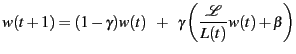
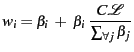
The window size computation uses a control mechanism shown to exhibit stable behavior for FAST TCP:

$$\vspace*{-0.05in} \abovedisplayskip \belowdisplayskip w(t+1) = (1- \gamma)w(t) \;\; + \;\; \gamma \left( \frac{\cal{L}}{L(t)}w(t) + \beta\right)$$ (2)

Here $w(t)$ denotes the window size at time $t$ , $\gamma \in [0,1]$ is a smoothing parameter, $\cal {L}$ is the system-wide latency threshold, and $\beta$ is a per-host parameter that reflects its IO shares allocation.

Whenever the average latency $L > \cal{L}$ , PARDA decreases the window size. When the overload subsides and $L < \cal{L}$ , PARDA increases the window size. Window size adjustments are based on latency measurements, which indicate load at the array, as well as per-host $\beta$ values, which specify relative host IO share allocations.

To avoid extreme behavior from the control algorithm, $w(t)$ is bounded by $[w_{min}, w_{max}]$ . The lower bound $w_{min}$ prevents starvation for hosts with very few IO shares. The upper bound $w_{max}$ avoids very long queues at the array, limiting the latency seen by hosts that start issuing requests after a period of inactivity. A reasonable upper bound can be based on typical queue length values in uncontrolled systems, as well as the array configuration and number of hosts.

The latency threshold $\cal {L}$ corresponds to the response time that is considered acceptable in the system, and the control algorithm tries to maintain the overall cluster-wide latency close to this value. Testing confirmed our expectation that increasing the array queue length beyond a certain value doesn't lead to increased throughput. Thus, $\cal {L}$ can be set to a value which is high enough to ensure that a sufficiently large number of requests can always be pending at the array. We are also exploring automatic techniques for setting this parameter based on long-term observations of latency and throughput. Administrators may alternatively specify $\cal {L}$ explicitly, based on cluster-wide requirements, such as supporting latency-sensitive applications, perhaps at the cost of under-utilizing the array in some cases.

Figure 2: Simulation of three hosts with $1:2:3$ share ratio. Array capacity is reduced from 400 to 100 req/s at $t$ = 100 s.

(a) Window size	(b) Average Latency	(c) Throughput

Finally, $\beta$ is set based on the IO shares associated with the host, proportional to the sum of its per-VM shares. It has been shown theoretically in the context of FAST TCP that the equilibrium window size value for different hosts will be proportional to their $\beta$ parameters [15].

We highlight two properties of the control equation, again relying on formal models and proofs from FAST TCP. First, at equilibrium, the throughput of host $i$ is proportional to $\beta_i/q_i$ , where $\beta_i$ is the per-host allocation parameter, and $q_i$ is the queuing delay observed by the host. Second, for a single array with capacity $C$ and latency threshold $\cal {L}$ , the window size at equilibrium will be:

$$\vspace*{-0.05in} w_i = \beta_i  +  \beta_i \frac{C{\cal{L}}}{\sum_{\forall {j}}\beta_{j}}$$ (3)

To illustrate the behavior of the control algorithm, we simulated a simple distributed system consisting of a single array and multiple hosts using Yacsim [17]. Each host runs an instance of the algorithm in a distributed manner, and the array services requests with latency based on an exponential distribution with a mean of $1/C$ . We conducted a series of experiments with various capacities, workloads, and parameter values.

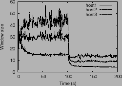
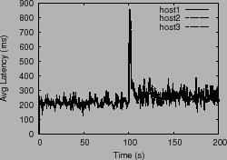
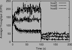
To test the algorithm's adaptability, we experimented with three hosts using a $1:2:3$ share ratio, $\cal {L}$ = 200 ms, and an array capacity that changes from 400 req/s to 100 req/s halfway through the experiment. Figure 2 plots the throughput, window size and average latency observed by the hosts for a period of $200$ seconds. As expected, the control algorithm drives the system to operate close to the desired latency threshold $\cal {L}$ . We also used the simulator to verify that as $\cal {L}$ is varied (100 ms, 200 ms and 300 ms), the system latencies operate close to $\cal {L}$ , and that windows sizes increase while maintaining their proportional ratio.