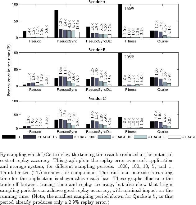
The causality engine can throttle every I/O issued by every node. However, sufficient replay accuracy can be obtained in significantly less time. In particular, one can sample across both dimensions (i.e., which I/Os to delay and which nodes to run in throttled mode). This experiment explores the first dimension, specifically the trade-off between replay accuracy and the I/O sampling period.
Five sampling periods are compared (1, 5, 10, 100, and 1000). As discussed in
Section 3, the period determines the frequency with which I/O
is delayed. If the sampling period is 1, every I/O is delayed. If the sampling
period is 5, every ![]() I/O is delayed, etc.
Given this, one would
expect the sampling period to have the greatest impact on applications with
a large number of I/O dependencies.
I/O is delayed, etc.
Given this, one would
expect the sampling period to have the greatest impact on applications with
a large number of I/O dependencies.
Note, I/O sampling can affect the computation calculation when using the throttling-based approach (Approach 1 in Section 3.2.1). Recall that throttling a node makes it slower than all the others. If the sampling frequency is too low (a large sampling period), then that node may not always be the slowest, thereby potentially introducing synchronization time into the trace which would be inadvertently counted as computation. Therefore, timing the system calls to determine computation time (Approach 2 in Section 3.2.2) is a more effective approach when using large sampling periods. None of the applications evaluated use ``untraceable'' mechanisms for synchronization, allowing Approach 2 to work effectively.
Figure 11 plots replay accuracy against the I/O sampling period, for each of the applications and storage systems being evaluated. Beginning with Pseudo, for which there are few data dependencies (i.e., all nodes must complete their last write before any node begins reading the checkpoint), one should expect little difference in replay error among the different sampling periods. As shown in the figure, the replay error for Pseudo is within 10% for all sampling periods and storage arrays.
PseudoSync and PseudoSyncDat behave quite differently (i.e., a barrier after every write I/O) and highlight the trade-off between tracing time and sampling period. As shown in the figure, replay error quickly decreases with smaller sampling periods. Notice the prominent staircase effect as the sampling is decreased from 1000 to 1. These applications represent the worst case scenario for sampling, where data dependencies are the primary factor influencing the replay rate.
Looking now at Fitness, one sees behavior very similar to Pseudo. Both have few data dependencies and do not require frequent I/O sampling for accurate replay. The error for Fitness is within 5% for all sampling periods.
Quake performance is influenced by synchronization (like PseudoSync and PseudoSyncDat). So, discovering more data dependencies offers improvements in replay accuracy. For example, an I/O sampling period of 5 yields a 2.9% replay error, compared to 21% error for an I/O sampling period of 1000.