
The key observation is that given the geometry and design of the
modern day disks, sequential bandwidth of the disks is
significantly higher (for example, more than ![]() times) than its
performance on 100% random write workload. The goal is to exploit
this differential by introducing spatial locality in the destage
order.
times) than its
performance on 100% random write workload. The goal is to exploit
this differential by introducing spatial locality in the destage
order.
This goal has been extensively studied in the context of disk scheduling algorithms. The key constraint in disk scheduling is to ensure fairness or avoid starvation that occurs when a disk I/O is not serviced for an unacceptably long time. In other words, the goal is to minimize the average response time and its variance. For detailed reviews on disk scheduling, see [23,24,25,26]. A number of algorithms are known: First-come-first-serve (FCFS) [27], Shortest seek time first (SSTF) [28] serves the I/O that leads to shortest seek, Shortest access time first (SATF), SCAN [28] serves I/Os first in increasing order and then in decreasing order of their logical addresses, Cyclical SCAN (CSCAN)[29] serves I/Os only in the increasing order of their logical addresses. There are many other variants known as LOOK [30], VSCAN [31], FSCAN [27], Shortest Positioning Time First (SPTF) [26], GSTF and WSTF [24], and Largest Segment per Track LST [11,32].
In the context of the present paper, we are interested in write
caching at an upper level in the memory hierarchy, namely, for a
storage controller. This context differs from disk scheduling in
two ways. First, the goal is to maximize throughput without
worrying about fairness or starvation for writes. This follows
since as far as the writer is concerned, the write requests have
already been completed after they are written in the NVS.
Furthermore, there are no reads that are being scheduled by the
algorithm. Second, in disk scheduling, detailed knowledge of the
disk head and the exact position of various outstanding writes
relative to this head position and disk motion is available. Such
knowledge cannot be assumed in our context. For example,
[21] found that applying SATF at a higher level was
not possible. They concluded that ``![]() we found that modern
disks have too many internal control mechanisms that are too
complicated to properly account for in the disk service time
model. This exercise lead us to conclude that software-based SATF disk schedulers are less and less feasible as the disk
technology evolves.'' Reference [21] further noted that
``Even when a reasonably accurate software-based SATF disk
scheduler can be successfully built, the performance gain over a
SCAN-based disk scheduler that it can realistically achieve
appears to be insignificant
we found that modern
disks have too many internal control mechanisms that are too
complicated to properly account for in the disk service time
model. This exercise lead us to conclude that software-based SATF disk schedulers are less and less feasible as the disk
technology evolves.'' Reference [21] further noted that
``Even when a reasonably accurate software-based SATF disk
scheduler can be successfully built, the performance gain over a
SCAN-based disk scheduler that it can realistically achieve
appears to be insignificant ![]() ''. The conclusions of
[21] were in the context of single disks, however, if
applied to RAID-5, their conclusions will hold with even more
force.
''. The conclusions of
[21] were in the context of single disks, however, if
applied to RAID-5, their conclusions will hold with even more
force.
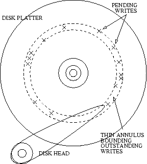
For these reasons, in this paper, we focus on CSCAN as the fundamental spatial locality algorithm that is suitable in our context. The reason that CSCAN works reasonably well is that at anytime it issues a few outstanding writes that all fall in a thin annulus on the disk, see, Figure 1. Hence, CSCAN helps reduce seek distances. The algorithm does not attempt to optimize for further rotational latency, but rather trusts the scheduling algorithm inside the disk to order the writes and to exploit this degree of freedom. In other words, CSCAN does not attempt to outsmart or outguess the disk's scheduling algorithm, but rather complements it.
 |
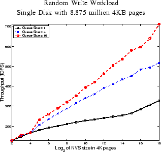 |
In Figure 2, we demonstrate that as the size of NVS managed by CSCAN grows, so does the achieved throughput. We use a workload that writes 4KB pages randomly over a single disk, and that has nearly 100% write misses. We also use several queue sizes that control the maximum number of outstanding writes that CSCAN can issue to the disk. It appears that throughput grows proportionally to the logarithm of the NVS size. As the size of NVS grows, assuming no starvation at the underlying disk, the average thickness of the annulus in Figure 1 should shrink - thus permitting a more effective utilization of the disk. Observe that the disks continuously rotate at a constant number of revolutions per second. CSCAN attempts to increase the number of writes that can be carried out per revolution.