WORLDS '05 Preliminary Paper [WORLDS '05 Technical Program]

Detecting Performance Anomalies in Global Applications

Terence Kelly
Hewlett-Packard Laboratories
1501 Page Mill Road m/s 1125
Palo Alto, CA 94304 USA

Abstract:

Understanding real, large distributed systems can be as difficult and important as building them. Complex modern applications that span geographic and organizational boundaries confound performance analysis in challenging new ways. These systems clearly demand new analytic methods, but we are wary of approaches that suffer from the same problems as the systems themselves (e.g., complexity and opacity).

This paper shows how to obtain valuable insight into the performance of globally-distributed applications without abstruse techniques or detailed application knowledge: Simple queueing-theoretic observations together with standard optimization methods yield remarkably accurate performance models. The models can be used for performance anomaly detection, i.e., distinguishing performance faults from mere overload. This distinction can in turn suggest both performance debugging tools and remedial measures.

Extensive empirical results from three production systems serving real customers--two of which are globally distributed and span administrative domains--demonstrate that our method yields accurate performance models of diverse applications. Our method furthermore flagged as anomalous an episode of a real performance bug in one of the three systems.

1 Introduction

Users and providers of globally-distributed commercial computing systems value application-level performance, because an unresponsive application can directly reduce revenue or productivity. Unfortunately, understanding application-level performance in complex modern distributed systems is difficult for several reasons. Today's commercial production applications are composed of numerous opaque software components running atop virtualized and poorly-instrumented physical resources. To make matters worse, applications are increasingly distributed across both geographical and organizational boundaries. Merely to collect in one place sufficient measurement data and knowledge of system design to support a detailed performance analysis is often very difficult in practice. Rapidly-changing application designs and configurations limit the useful life-span of an analysis once it has been performed.

For these reasons operators and administrators seldom analyze running production systems except in response to measurements (or user complaints) indicating unacceptably poor performance. The analyst's task is simplified if she can quickly determine whether the problem is due to excessive workload. If so, the solution may be as simple as provisioning additional resources for the application; if not, the solution might be to ``reboot and pray.'' If such expedients are not acceptable and further analysis is required, knowing whether workload accounts for observed performance can guide the analyst's choice of tools: Ordinary overload might recommend resource bottleneck analysis, whereas degraded performance not readily explained by workload might suggest a fault in application logic or configuration. If different organizations manage an application and the systems on which it runs, quickly determining whether workload accounts for poor performance can decide who is responsible for fixing the problem, averting finger-pointing. In summary, performance anomaly detection--knowing when performance is surprising, given workload--does not directly identify the root causes of problems but can indirectly aid diagnosis in numerous ways.

Table: Summary of data sets and model quality.

Data	collection		number of	# trans'n	$\sum_i\vert e_i\vert / \sum_i y_i$
set	dates	duration	transactions	types	OLS	LAR
ACME	July 2000	4.6 days	159,247	93	.2154	.1968
FT	Jan 2005	31.7 days	5,943,847	96	.1875	.1816
VDR	Jan 2005	10.0 days	466,729	37	.1523	.1466

This paper explores a simple approach to explaining application performance in terms of offered workload. The method exploits four properties typical of commercially-important globally-distributed production applications:

1.: workload consists of request-reply transactions;
2.: transactions occur in a small number of types (e.g., ``log in,'' ``browse,'' ``add to cart,'' ``check out'' for an E-commerce site);
3.: resource demands vary widely across but not within transaction types;
4.: computational resources are adequately provisioned, so transaction response times consist largely of service times, not queueing times.

We shall see that for applications with these properties, aggregate response time within a specified period is well explained in terms of transaction mix.

Our empirical results show that models of aggregate response time as a simple function of transaction mix have remarkable explanatory power for a wide variety of real-world distributed applications: Nearly all of the time, observed performance agrees closely with the model. The relatively rare cases where actual performance disagrees with the model can reasonably be deemed anomalous. We present a case study showing that our method identified as anomalous an episode of an obscure performance fault in a real globally-distributed production system.

Performance anomaly detection is relatively straightforward to evaluate and illustrates the ways in which our approach complements existing performance analysis methods, so in this paper we consider only this application of our modeling technique. Due to space constraints we do not discuss other applications, e.g., capacity planning and resource allocation.

2 Transaction Mix Models

We begin with a transaction log that records the type and response time of each transaction. We divide time into intervals of suitable width (e.g., 5 minutes for all experiments in this paper). For interval $i$ let $N_{ij}$ denote the number of transactions of type $j$ that began during the interval and let $T_{ij}$ denote the sum of their response times. We consider models of the form

$\begin{displaymath} y_i \ \ = \ \ \sum_j T_{ij} \ \ = \ \ \alpha_1 N_{i1} + \alpha_2 N_{i2} + \cdots \end{displaymath}$

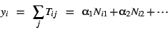(1)

Note that no intercept term is present in Equation

, i.e., we constrain the model to pass through the origin: aggregate response time must be zero for intervals with no transactions. For given vectors of model parameters $a_j$ and observed transaction mix $N_{ij}$ at time $i$ , let

$\begin{displaymath} \hat{y}_i \ \ = \ \ f_{\vec{a}}(\vec{N}_i) \ \ = \ \ \sum_j a_j N_{ij} \end{displaymath}$

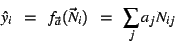(2)

denote the fitted value of the model at time $i$ and let $e_i \ \ = \ \ y_i - \hat{y}_i$ denote the residual (model error) at time $i$ . We define the accuracy of a model as a generalization of the familiar concept of relative error:

$\begin{displaymath} \mathrm{normalized \ aggregate \ error} \ \equiv \ \frac{\sum_i \vert e_i\vert}{\sum_i y_i} \end{displaymath}$

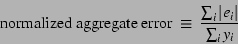(3)

We say that a model of the form given in Equation

is optimal if it minimizes the figure of merit in Equation

. We shall also report the distribution of residuals and scatterplots of $(y, \hat{y})$ pairs for our models. (The coefficient of multiple determination $R^2$ cannot be used to assess model quality; it is not meaningful because Equation

lacks an intercept term [17, p. 163].)

To summarize, our methodology proceeds through the following steps: 1) obtain parameters $a_j$ by fitting the model of Equation to a data set of transaction counts $N_{ij}$ and response times $T_{ij}$ ; 2) feed transaction counts $N_{ij}$ from the same data set into Equation to obtain fitted values $\hat{y}_i$ ; 3) compare fitted values $\hat{y}_i$ with observed values $y_i$ to assess model accuracy; 4) if the $\hat{y}_i$ agree closely with the corresponding $y_i$ for most time intervals $i$ , but disagree substantially for some $i$ , deem the latter cases anomalous. We emphasize that we do not divide our data into ``training'' and ``test'' sets, and that our goal is not to forecast future performance. Instead, we retrospectively ask whether performance can be explained well in terms of offered workload throughout most of the measurement period. If so, the rare cases where the model fails to explain performance may deserve closer scrutiny.

Numerous methods exist for deriving model parameters $a_j$ from data. The most widely-used procedure is ordinary least-squares (OLS) multivariate regression, which yields parameters that minimize the sum of squared residuals $\sum_i e_i^2$ [17]. Least-squares regression is cheap and easy: it is implemented in widely-available statistical software [18] and commercial spreadsheets (e.g., MS Excel). However it can be shown that OLS models can have arbitrarily greater normalized aggregate error than models that minimize Equation , and therefore we shall also compute the latter. Optimal-accuracy model parameters minimize the sum of absolute residuals $\sum_i \vert e_i\vert$ . The problem of computing such parameters is known as ``least absolute residuals (LAR) regression.'' LAR regression requires solving a linear program. We may employ general-purpose LP solvers [15] or specialized algorithms [4]; the computational problem of estimating LAR regression parameters remains an active research area [11].

Statistical considerations sometimes recommend one or another regression procedure. For instance, OLS and LAR provide maximum-likelihood parameter estimates for different model error distributions. Another important difference is that LAR is a robust regression procedure whereas OLS is not: A handful of outliers (extreme data points) can substantially influence OLS parameter estimates, but LAR is far less susceptible to such distortion. This can be an important property if, for instance, faulty measurement tools occasionally yield wildly inaccurate data points. In this paper we shall simply compare OLS and LAR in terms of our main figure of merit (Equation ) and other quantities of interest.

Intuitively, for models that include all transaction types $j$ and for data collected during periods of extremely light load, parameters $a_j$ represent typical service times for the different transaction types. Interaction effects among transactions are not explicitly modeled, nor are waiting times when transactions queue for resources such as CPUs, disks, and networks. Our ongoing work seeks to amend the model of Equation with terms representing waiting times. This is not straightforward because the multiclass queueing systems that we consider are much harder to analyze than single-class systems [5] (classes correspond to transaction types). As we shall see in Section , the severe simplifying assumptions that we currently make do not preclude remarkable accuracy.

Well-known procedures exist for simplifying models such as ours, but these must be used with caution. The number of transaction types can be inconveniently large in real systems, and a variety of refinement procedures are available for reducing in a principled way the number included in a model [17]. When we reduce the number of transaction types represented, however, parameters $a_j$ no longer have a straightforward interpretation, and negative values are often assigned to these parameters. On the other hand, the reduced subset of transaction types selected by a refinement procedure may represent, loosely speaking, the transaction types most important to performance. Model refinement therefore provides an application-performance complement to procedures that automatically identify utilization metrics most relevant to performance [12]. We omit results on model refinement due to space limitations.

Measuring our models' accuracy is easy, but evaluating their usefulness for performance anomaly detection poses special challenges. If a model is reasonably accurate in the sense that observed performance $y_i$ is close to the fitted value $\hat{y}_i$ for most time intervals $i$ , why should we regard the relatively rare exceptions as ``anomalous'' or otherwise interesting? To address this question we model data collected on systems with known performance faults that occur at known times and see whether the model fails to explain performance during fault episodes.

3 Empirical Evaluation

**Figure:** The globally-distributed ``FT'' application.
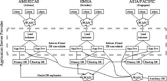$\begin{figure}\centerline{\psfig{figure=FIGS/newesarch02.eps,width=\columnwidth}}\end{figure}$

We evaluate the method of Section using three large detailed data sets collected on real production systems. The first, which we call ``ACME,'' was collected in July 2000 on one of several servers comprising a large Web-based shopping system; see Arlitt et al. for a detailed workload characterization [2]. The other two, which we call ``FT'' and ``VDR,'' were collected in early 2005 on two globally-distributed enterprise applications serving both internal HP users and external customers. Cohen et al. provide a detailed description of FT [13]; VDR shares some features in common with FT but has not been analyzed previously. One noteworthy feature common to both FT and VDR is that different organizations are responsible for the applications and for the application-server infrastructure on which they run. Figure sketches the architecture of the globally-distributed FT application; a dashed rectangle indicates managed application servers.

**Figure:** Cumulative distribution of $\vert e_i\vert/y_i$ , FT data.
$\begin{figure}\centerline{\psfig{figure=FIGS/hpat615_resid_cdf.eps, width=\columnwidth}}\end{figure}$

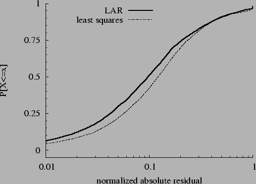Table describes our three data sets and presents summary measures of model quality for least-squares and LAR parameter estimation. Our figure of merit from Equation , $\sum_i\vert e_i\vert / \sum_i y_i$ , shows that the models are quite accurate. In all cases, for LAR regression, normalized aggregate error ranges from roughly 15% to under 20%. Least-squares regression yields slightly worse models by this measure; it increases $\sum_i \vert e_i\vert$ by 3.2%-9.5% for our data. Figure shows the cumulative distribution of absolute residuals normalized to $y$ , i.e., the distribution of $\vert e_i\vert/y_i$ , for the FT data and both regression procedures. The LAR model is wrong by 10% or less roughly half of the time, and it is almost never off by more than a factor of two. The figure also shows that LAR is noticeably more accurate than least-squares.

**Figure:** Scatterplot of $y_i$ vs. $\hat{y}_i$ , FT data.
$\begin{figure}\centerline{\psfig{figure=FIGS/LSQ_HPAT615_JAN.eps, width=\columnwidth}}\end{figure}$

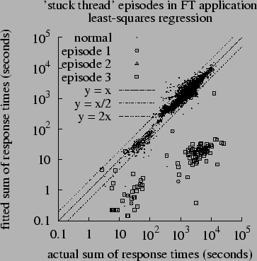A scatterplot of fitted vs. observed aggregate response times offers further insight into model quality. Figure shows such a plot for the FT data and OLS regression. Plots for LAR regression and other data sets are qualitatively similar: Whereas aggregate response times $y$ range over several orders of magnitude, in nearly all cases fitted values $\hat{y}$ differ from $y$ by less than a factor of two. A small number of points appear in the lower-right corner; these represent time intervals whose observed aggregate response times were far larger than fitted model values. For our data sets, the reverse is very rare, and very few points appear in the upper-left corner. Such points might indicate that transactions are completing ``too quickly,'' e.g., because they quickly abort due to error.

As the FT data of Figure was being collected, there occurred several episodes of a known performance fault that was eventually diagnosed and repaired. This fault, described in detail in [13], involved an application misconfiguration that created an artificial bottleneck. An important concurrency parameter in the application server tier, the maximum number of simultaneous database connections, was set too low. The result was that queues of worker threads waiting for database connections in the app server tier grew very long during periods of heavy load, resulting in excessively--and anomalously--long transaction response times. FT operators do not know precisely when this problem occurred because queue lengths, waiting times, and utilization are not recorded for finite database connection pools and other ``soft'' resources. However the admins gave us rough estimates that allow us to identify three major suspected episodes, shown with special points in Figure .

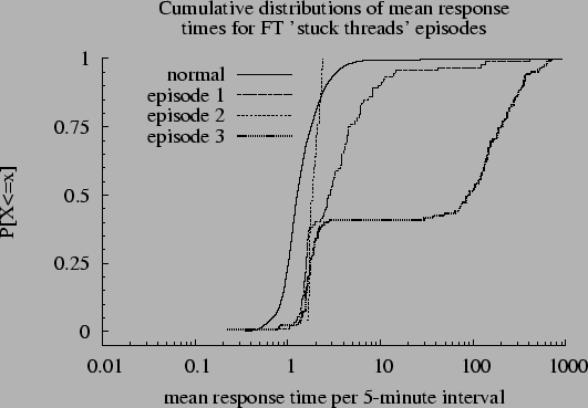
**Figure:** CDFs of mean response times during ``stuck threads'' episodes.
$\begin{figure}\centerline{\psfig{figure=FIGS/HPAT615_JAN_MEANRESP.eps, width=\columnwidth}}\end{figure}$

The most remarkable feature of the figure is that false positives are extremely rare: Data points for ``normal'' time intervals are almost never far from the $y = x$ diagonal and nearly all large discrepancies between $y$ and $\hat{y}$ occur during suspected performance fault episodes. Unfortunately, false negatives do seem evident in the figure: Of the three suspected performance fault episodes, only episode 3 (indicated by open squares) appears far from $y = x$ ; most points corresponding to episodes 1 and 2 lie near the diagonal. Has our method failed to detect performance anomalies, or does the problem reside in our inexact conjectures regarding when episodes occurred? Figure suggests the latter explanation. This figure shows the distributions of average (as opposed to aggregate) transaction response times for four subsets of the FT data: normal operation and the three alleged performance fault episodes. Figure shows that episode 3--the one that stands out in Figure --has far higher mean response times than the other two episodes.

Several explanations are possible for our results. One possibility is that the problem did in fact occur during all three alleged episodes, and that our proposed anomaly detection method identifies only the most extreme case. Another possibility is that alleged episodes 1 and 2 were not actual occurrences of the problem. Based on how the alleged episodes were identified, and based on the large difference between episode 3 and the other two in Figure , the latter explanation seems more likely. (In a similar vein, Cohen et al. report that an episode of this problem on a host not analyzed here was initially mis-diagnosed [13].) For our ongoing work we hope to analyze systems with sporadic performance faults whose episodes are known with greater certainty. Data on such systems is hard to obtain, but it is required for a compelling evaluation of the proposed method.

4 Discussion

Section shows that the very simple transaction mix performance models of Section have remarkable explanatory power for real, globally-distributed production systems; they furthermore sometimes flag subtle performance bugs as anomalous. We would expect our technique to work well for any system that approximately conforms to the simplifying assumptions enumerated in Section : Workload consists of transactions that fall into a small number of types; service times vary less within types than across types; and resources are adequately provisioned so that service times dominate response times. This section discusses limitations inherent in our assumptions, the usefulness of the proposed method, and extensions to broaden its applicability.

We can identify plausible scenarios where our assumptions fail and therefore our method will likely perform poorly. If workload is moderately heavy relative to capacity, queueing times will account for an increasing fraction of response times, and model accuracy will likely suffer. We would also expect reduced accuracy if service times are inter-dependent across transaction types (e.g., due to resource congestion). For instance, ``checkout'' transactions may require more CPU time during heavy browsing if the latter reduces CPU cache hit rates for the former.

On the positive side, our method does not suffer if transactions are merely numerous, internally complex, or opaque. Furthermore it may flag as anomalous situations where problems are actually present but our simplifying assumptions are not violated. For instance, it can detect cases where transactions complete ``too quickly,'' e.g., because they abort prematurely. Finally, our method can be used to detect anomalies in real time. At the close of every time window (e.g., every five minutes) we simply fit a model to all available data (e.g., from the previous week or month) and check whether the most recent data point is anomalous. LAR and OLS regressions may be computed in less than one second for the large data sets of Table .

Our ongoing work extends the transaction mix model of Equation with additional terms representing queueing time. A naïve approach is simply to add resource utilization terms as though they were transaction types. Our future work, however, will emphasize more principled ways of incorporating waiting times, based on queueing theory. Perhaps the most important aspect of our ongoing work is to validate our methods on a wider range of real, large distributed systems. Testing model accuracy requires only transaction types and response times, which are relatively easy to obtain. However to verify that performance anomalies reported by our models correspond to performance bugs in real systems requires reliable information about when such bugs occurred, and such data is difficult to obtain.

5 Related Work

Researchers have proposed statistical methods for performance anomaly detection in a variety of contexts. Chen et al. [10] and Kiciman & Fox [16] use fine-grained probabilistic models of software component interactions to detect faults in distributed applications. Ide & Kashima analyze time series of application component interactions; their method detected injected faults in a benchmark application serving synthetic workload [14]. Brutlag describes a far simpler time-series anomaly detection method [6] that has been deployed in real production systems for several years [7]. Our approach differs in that it exploits knowledge of the transaction mix in workload and does not employ time series analysis; it is also far simpler than most previous methods.

If a performance problem has been detected and is not due to overload, one simple remedial measure is to re-start affected application software components. Candea & Fox argue that components should be designed to support deliberate re-start as a normal response to many problems [8]. Candea et al. elaborate on this theme by proposing fine-grained rebooting mechanisms [9].

On the other hand, if workload explains poor performance, a variety of performance debugging and bottleneck analysis tools may be applied. Barham et al. exploit detailed knowledge of application architecture to determine the resource demands of different transaction types [3]. Aguilera et al. and Cohen et al. pursue far less knowledge-intensive approaches to detecting bottlenecks and inferring system-level correlates of application-level performance [12,1]. Cohen et al. later employed their earlier techniques in a method for reducing performance diagnosis to an information retrieval problem [13]. The performance anomaly detection approach described in this paper may help to inform the analyst's choice of available debugging tools.

Queueing-theoretic performance modeling of complex networked services is an active research area. Stewart & Shen predict throughput and mean response time in such services based on component placement and performance profiles constructed from extensive benchmarking [19]. They use a single-class M/G/1 queueing expression to predict response times. Urgaonkar et al. describe a sophisticated queueing network model of multi-tier applications [20]. This model requires rather extensive calibration, but can be used for dynamic capacity provisioning, performance prediction, bottleneck identification, and admission control.

6 Conclusions

We have seen that very simple transaction mix models accurately explain application-level performance in complex modern globally-distributed commercial applications. Furthermore, performance faults sometimes manifest themselves as rare cases where our models fail to explain performance accurately. Performance anomaly detection based on our models therefore appears to be a useful complement to existing performance debugging techniques. Our method is easy to understand, explain, implement, and use; an Apache access log, a bit of Perl, and a spreadsheet suffice for a bare-bones instantiation. Our technique has no tunable parameters and can be applied without fuss by nonspecialists; in our experience it always works well ``out of the box'' when applied to real production systems.

More broadly, we argue that a principled synthesis of simple queueing-theoretic insights with an accuracy-maximizing parameter estimation procedure yields accurate and versatile performance models. We exploit only limited and generic knowledge of the application, namely transaction types, and we rely on relatively little instrumentation. Our approach represents a middle ground between knowledge-intensive tools such as Magpie on the one hand and nearly-knowledge-free statistical approaches on the other. Our future work explores other topics that occupy this interesting middle ground, including extensions of the method described here.

7 Acknowledgments

I thank Alex Zhang and Jerry Rolia for useful discussions of queueing theory, and statistician Hsiu-Khuern Tang for answering many questions about LAR regression and other statistical matters. Sharad Singhal, Jaap Suermondt, Mary Baker, and Jeff Mogul reviewed early drafts of this paper and suggested numerous improvements; WORLDS reviewers supplied similarly detailed and valuable feedback. The anonymous operators of the ACME, FT, and VDR production systems generously allowed researchers access to measurements of their system, making possible the empirical work of this paper. Researchers Martin Arlitt, Ira Cohen, Julie Symons, and I collected the data sets. Fereydoon Safai provided access to the linear program solver used to compute LAR parameters. Finally I thank my manager, Kumar Goswami, for his support and encouragement.

Bibliography

1: M. K. Aguilera, J. C. Mogul, J. L. Wiener, P. Reynolds, and A. Muthitacharoen.
Performance debugging for distributed systems of black boxes.
In Proc. SOSP, pages 74-89, Oct. 2003.
2: M. Arlitt, D. Krishnamurthy, and J. Rolia.
Characterizing the scalability of a large web-based shopping system.
ACM Trans. on Internet Tech, 1(1):44-69, Aug. 2001.
3: P. Barham, A. Donnelly, R. Isaacs, and R. Mortier.
Using Magpie for request extraction and workload modelling.
In Proc. OSDI, pages 259-272, Dec. 2004.
4: I. Barrodale and F. Roberts.
An improved algorithm for discrete L1 linear approximations.
SIAM Journal of Numerical Analysis, 10:839-848, 1973.
5: G. Bolch, S. Greiner, H. de Meer, and K. S. Trivedi.
Queueing Networks and Markov Chains.
Wiley, 1998.
6: J. Brutlag.
Aberrant behavior detection in time series for network service monitoring.
In USENIX System Admin. Conf. (LISA), pages 139-146, Dec. 2000.
7: J. Brutlag.
Personal communication, Mar. 2005.
8: G. Candea and A. Fox.
Crash-only software.
In Proc. HotOS-IX, May 2003.
9: G. Candea, S. Kawamoto, Y. Fujiki, G. Friedman, and A. Fox.
Microreboot: A technique for cheap recovery.
In Proc. OSDI, Dec. 2004.
10: M. Y. Chen, A. Accardi, E. Kiciman, D. Patterson, A. Fox, and E. Brewer.
Path-based failure and evolution management.
In Proc. NSDI, Mar. 2004.
11: K. L. Clarkson.
Subgradient and sampling algorithms for $l_1$ regression.
In Proc. 16th ACM-SIAM Symposium on Discrete Algorithms (SODA), pages 257-266, 2005.
12: I. Cohen, M. Goldszmidt, T. Kelly, J. Symons, and J. S. Chase.
Correlating instrumentation data to system states: A building block for automated diagnosis and control.
In Proc. OSDI, Oct. 2004.
13: I. Cohen, S. Zhang, M. Goldszmidt, J. Symons, T. Kelly, and A. Fox.
Capturing, indexing, clustering, and retrieving system history.
In Proc. SOSP, Oct. 2005.
14: T. Ide and H. Kashima.
Eigenspace-based anomaly detection in computer systems.
In Proc. SIGKDD, Aug. 2005.
15: ILOG Corporation.
CPLEX and related software documentation.
https://www.ilog.com.
16: E. Kiciman and A. Fox.
Detecting application-level failures in component-based internet services.
IEEE Transactions on Neural Networks, Spring 2005.
17: J. Neter, M. H. Kutner, C. J. Nachtsheim, and W. Wasserman.
Applied Linear Statistical Models.
Irwin, fourth edition, 1996.
18: The R statistical software package, Apr. 2005.
https://www.r-project.org/.
19: C. Stewart and K. Shen.
Performance modeling and system management for multi-component online services.
In Proc. NSDI, pages 71-84, 2005.
20: B. Urgaonkar, G. Pacifici, P. Shenoy, M. Spreitzer, and A. Tantawi.
An analytical model for multi-tier internet services and its applications.
In Proc. ACM SIGMETRICS, pages 291-302, June 2005.

About this document ...

Detecting Performance Anomalies in Global Applications

This document was generated using the LaTeX2HTML translator Version 2002 (1.62)

The command line arguments were:
latex2html -split 0 -show_section_numbers -local_icons anomdet.tex

The translation was initiated by on 2005-10-06

Footnotes

... Applications: Second Workshop on Real, Large Distributed Systems (WORLDS), San Francisco, 13 December 2005.
$\usebox{\confurl}$
$\usebox{\rcsid}$

2005-10-06

Need help?

Last changed: 24 Oct. 2005 jel