|
Abstract Performance problems in complex systems are often caused by under-provisioning, workload interference, incorrect expectations or bugs. Troubleshooting such systems is a difficult task faced by service engineers. We have built CLUEBOX, a non-intrusive toolkit that aids rapid problem diagnosis. It employs machine learning techniques on the available performance logs to characterize workloads, predict performance and discover anomalous behavior. By identifying the most relevant anomalies to focus on, CLUEBOX automates the most onerous aspects of performance troubleshooting. We have experimentally validated our methodology in a networked storage environment with real workloads. Using CLUEBOX to learn from a set of historical performance observations, we were able to distill over 2000 performance counters into 68 counters that succinctly describe a running workload. Further, we demonstrate effective troubleshooting of two scenarios that adversely impacted application response time: (1) an unknown competing workload, and (2) a file system consistency checker. By reducing the set of anomalous counters to examine to a dozen significant ones, CLUEBOX was able to guide a systems engineer towards identifying the correct root-cause rapidly. |
Enterprise data centers contain large, complex systems whose performance behavior is difficult to characterize. The vendors of these systems get many performance-related service calls from the users. The causes of the problem could be one of many. Under-provisioning, where the system is not able to handle the workload, is a common cause. Another cause of a perceived performance problem is that of interfering workloads. Often, the administrator will not be aware of the various background activities such as disk scrubs, RAID reconstructions, anti-virus scans, and data replication. As a result, the main application workload may suffer intolerable response time or throughput. Bugs are yet another cause of performance problems.
The above scenarios often manifest themselves primarily as one thing – a slowing down of the application. Someone has to piece together a variety of hidden symptoms and arrive at a diagnosis. Troubleshooting is an expert-intensive activity. It is also a time-sensitive activity – the longer it takes to identify and to solve a problem, the costs mount. Therefore, there is a real need for an automated facility for troubleshooting. In this paper, we make significant inroads into this area. The contributions of this paper are as follows.
The rest of the paper is organized as follows. Section 2 presents the current state of research in this area and places our work in context. Section 3 describes the architecture of our machine learning toolkit and describes how it crafts a workload signature, predicts latencies and identifies anomalies. Section 4 offers experimental validation of our techniques. Section 5 summarizes the lessons learned and proposes avenues for continuing this work. Finally, Section 6 presents our conclusions.
In the past few years, the systems research community has come to understand that quick diagnosis and repair of complex computer systems is beyond the capabilities of human administrators [12]. As a first step towards automated troubleshooting, rule-based expert systems have been proposed [13]. We believe that this approach is difficult to sustain. Systems evolve, workloads change, and having to involve an expert constantly to update the rules is not scalable. Therefore, there has been significant research into statistical learning systems for tackling this problem.
Systems such as PinPoint [5] and Magpie [2] diagnose problems in distributed systems by monitoring the communications between black box components or by inferring causal paths by analyzing message-level traces[1]. Spectroscope [17] is another system that uses clustering on request flow graphs constructed from traces, to categorize and to learn about differences in system behavior. Pip [16] proposes formalisms to allow programmers to express expectations about systems’ communication, timing and resource consumption, using a declarative language. In contrast to Pip and PinPoint, we do not seek to derive causality directly. Unlike the kind of applications that they seek to model such as web services and EJBs, our problem domain is large systems such as servers and storage. We use performance logs collected by a system as opposed to tracing communication. The methodologies are complementary.
Recent work has explored using Tree-Augmented Bayesian Networks for analyzing counter data [6], as well as extending the work to include ensembles of models [18] to characterize good workload execution and anomalous execution. They report that models serve well to identify SLO violations in web services. Unlike our work, their models have to be trained with both normal and bad behavior, and are able to identify only those anomalous behaviors that the models know about. They also do not have predictive capabilities like ours. Another work on statistical debugging in a Microsoft environment [3] attempts to discover which process is at fault in end-user environments. The complexity of the system and the instrumentation data that we are attempting to characterize is much higher.
An interesting approach towards root-cause analysis of problems in replicated systems [15] is to combine local (node-level) anomaly detection with global analysis. The intuition here is that the node with a different view of the anomalies when compared with the other nodes is the root-cause. The granularity of the anomaly is a node, and they report modest success in their results.
We do not invent new mathematical techniques in this paper. We use existing data mining techniques and compose them in an innovative way to implement an end-to-end system for performance troubleshooting.
The methodology used in CLUEBOX translates to a variety
of systems. However, we will present it in the context of a
network storage controller or a NAS appliance. The storage
controller consists of processors and disks organized in
RAID groups; it serves data to clients via network file system
protocols like NFS and CIFS. Data is stored in containers
called volumes that reside on disks. Data from clients
is stored using a file system called WAFL [8]. The
complex storage controller software has been instrumented
over the years with a large set of performance counters,
which are periodically dumped into a performance log.
There are counters that measure the number of ops/sec,
latencies, utilizations, etc. Many of these counters are
correlated with each other. Some counters compose
information from lower layers. Not only are there a lot of
counters, they have also evolved over time. Different
components log these statistics at different times and
frequencies. This is typical of large complex systems. We
used the R environment [9] for statistical computing and
graphics. We describe our techniques in the following
sections.
[8]. The
complex storage controller software has been instrumented
over the years with a large set of performance counters,
which are periodically dumped into a performance log.
There are counters that measure the number of ops/sec,
latencies, utilizations, etc. Many of these counters are
correlated with each other. Some counters compose
information from lower layers. Not only are there a lot of
counters, they have also evolved over time. Different
components log these statistics at different times and
frequencies. This is typical of large complex systems. We
used the R environment [9] for statistical computing and
graphics. We describe our techniques in the following
sections.
|
First, we attempt to understand the effect of workloads on a system. In the abstract, workloads have two dimensions: a characteristic and an intensity. The characteristic of a workload refers to attributes such as the read/write ratio, sequentiality, and arrival distribution. The intensity of a workload refers to attributes such as the arrival rate of operations and throughput of data read. CLUEBOX is a modeling tool that analyzes performance logs and learns about the characteristics of the workloads. Further, having been trained with workloads of varied characteristics and intensities, CLUEBOX is able to predict the performance of a given workload, spot a performance problem, and identify the few anomalous counters that could help an engineer rapidly identify the root-cause of the issue. In this section, we detail our learning methodology.
Clustering algorithms do not perform well if the number of features (counters) is large. Therefore, dimension reduction techniques are often applied as a data pre-processing step. The instance of the storage controller that we have been performing our experiments on, logs more than 2000 counters. It is computationally impractical to use the entire set for clustering or classification. Many counters have little information value but hamper effective analysis by adding noise. A standard method for dimensionality reduction is called Principal Component Analysis (PCA) [7]. Since PCA loses the intuitive meaning of the counters, we chose to use a method called Principal Feature Analysis (PFA) [14]. By using PFA, we reduced our counter set to around 300 for the type of workloads that are described in Tables 1 and 2.
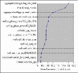
To distill the counters further requires a different kind of analysis. In any counter set, some of the counters are more important to characterizing the workload than others. We use a standard machine learning technique called random forest (RF) [4], which uses decision trees to classify labeled data. The output of the RF unsupervised learning algorithm gives us a ranking of the counters by their importance in classifying the observations, as shown in Figure 1.
Given the ranked list of counters, we now figure out the cutoff point beyond which the information value of the counters is low. We use clustering using CLARA [11] for that purpose. By clustering on increasing subsets of the ranked counters, we discover the smallest set of counters that distinguishes the workloads most effectively. Algorithm 1 has the details. In our experiments, described in Section 4.1, the top 68 counters distinguished the workloads the best. We call this counter set the workload signature profile. A cluster contains points representing all intensities of a given workload characteristic. The signature of a given workload is the medoid of its cluster as calculated above, and serves as a concise description of the workload. Note that the signature is dependent on the training set. By making the training set encompass the type of workloads that the system is expected to encounter, we can be confident that the signature does not miss important counters. Typically, a given system in an enterprise deployment will see only a few workload types corresponding to the applications that are used, so the performance logs of a running system should have adequate data for training.
|
The performance of the system when a given workload is imposed on it depends on the characteristic and the intensity of the workload. For simplicity, we assume that the average system latency of NFS operations represents the performance of the system. The scheme is extendable to other metrics such as throughput. CLUEBOX is trained with workloads at various intensities and the latencies are recorded for each cluster (i.e., workload signature) at each intensity. Decision tree modeling based on RF regression analysis is then used for performance prediction. Given an input workload, CLUEBOX will generate a predicted average system latency.
We next explain how the model can be used for detecting anomalous system behavior.
We assume that the user articulates his issue in the following form: “The performance of the system was fine at time T. I haven’t changed a thing since then, but now the latencies are unacceptably high.”
First, we have to discover the workload that is running on the system. Because of the perceived performance problem, current data cannot be used for this task since the counter values may not match the workload that the user thinks he is running. We therefore use data from time T to identify the workload. We could have also worked backwards in time to find a workload that’s known to the model.
When the vector of counter values at time T is given to CLUEBOX, its first job is to identify the current running workload by matching it against known workloads. We perform this step as follows.
Every known workload belongs to a cluster whose medoid represents the signature of that workload. CLUEBOX creates an RF using the medoids and the test workload. Passing the test data and the medoids through the decision trees of the RF, it calculates the proximity between the test data and the medoids. The medoid that has the highest proximity to the test load is considered to be the closest workload cluster. We now have to discover the intensity. A comprehensive set of logs will include each workload type at varying intensities. The RF of the closest workload cluster will encode data points from the workload at different intensities. The RF computes proximity measures between these observations and the counter values at time T. If the proximity measure is close to 1, then we infer that the test load is of known intensity; if the proximity measure is close to 0, then we infer that it is of unknown intensity. If the intensity of the test load is unknown, we use interpolation in our prediction model.
Next, the random forest of the closest workload is extracted. The test load is run through the decision trees of the random forest to generate a prediction for the average latency.
CLUEBOX compares the predicted system latency Lp with the observed latency Lo. The user can set a threshold value of deviation, Lt, of the predicted latency from the observed latency. When |Lp -Lo|∕Lp > Lt, it flags the corresponding observation as a suspect for an anomaly. Based on the closest workload characteristic and intensity, it generates a table containing the observed value of the counter, the expected value of the counter and the deviation between them.
There are two dimensions to anomaly detection: 1) the sensitivity of latencies to each of the counter values, and 2), the degree of deviation between the expected and observed values for each of the counters. CLUEBOX first examines the counters in the order of the importance value of the counter within the given workload, which is generated during the construction of the random forest. The importance value describes the sensitivity of a system output metric of interest (in this paper, the average latency) to that particular variable. If the top counters in the table show a major deviation, they are likely to be the key anomalies.
The tool then examines the counters based on the error between the observed counter value and the expected counter value. This helps in identifying which counter is affected the most. The tool takes both the error and importance value into account to come up with a ranked list of anomalous counters that could identify the root-cause of the performance problem. Algorithm 2 gives an outline of the method.
|
In this section, we present our evaluation of CLUEBOX along three lines – inferring workload signatures from performance logs, matching new workloads against known signatures, and narrowing down the root cause of anomalous behavior.
We ran each workload for 3 hours from a remote NFS client. Between each workload run, we restored the system to a common state using SnapshotTMtechnology in the storage controller. The storage controller was a FAS960 model having 6 GB of memory and six disks in a RAID-DP configuration. Tables 1 and 2 show details of each workload.
|
During the run, we collected performance logs at 1-minute intervals. Then, we coalesced the collected data into a single time-series data set of counter value vectors. Subsequently, we removed counters (columns) that were zero all the time and performed PFA to remove redundant counters. This step reduced the number of counters to analyze to 309. Using the RF Unsupervised Learning algorithm, we then ranked the counters in order of their importance towards quantifying the dissimilarities between the data points. Finally, we clustered the data set based on top-ranked N counters to determine the “sweet spot” – the ideal number of counters that will distinguish our workloads most effectively. Table 3 displays our results for increasing values of N.
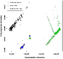
We see that when the top 40 counters are used for clustering, the namespace-intensive workloads separate from I/O-intensive workloads, but we get no further separation. When we increase the number of counters to 51, PostMark and Cthon workloads form distinct clusters. Using 57 counters gives us separate clusters for reads and writes; using 62 counters distinguishes random reads, random writes, sequential reads and sequential writes, as well as individual Sysbench workloads. Clustering using the top 68 counters gives us the expected ideal result, where each of our distinctly different workloads falls into different clusters. Workloads that are similar, such as S1 and S5, naturally do not exhibit any separation, which is an expected outcome. We also found that using more counters reduces the quality of clustering because the data gets noisier. The standard 2-D projection scatter plot of three of the workload clusters in Figure 3 offers visual confirmation that our clustering is good. We note that for our evaluation, we manually inspect the clustering output to identify if it is ideal. We conjecture that we could automate this step in the future by using well-known clustering quality metrics.
|
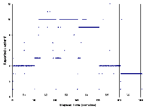
We show the quality of the clustering of SIO workloads in Figure 2. As we can see, Cluster 4 is composed of points from S1 and S5, which are very similar sequential read workloads. Cluster 10 is composed of points from S2 and S3, which are similar sequential write workloads. S4, a random write workload, clearly separates out. So does S6, a random read workload. Cluster 5 has a few stray points from many workloads; these points represent the beginning stages of workloads where the state of the system is “cold.”‘
Since our experiments involved a wide variety of workloads, we are confident that these 68 counters clearly define the effect of running a workload on our system, and will serve as the workload signature profile of the system.
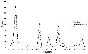
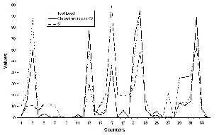
To see how well CLUEBOX detects the similarity of a running workload with known workloads (identified in Table 1), we ran a test SIO workload with 90% reads, 80% of them being sequential. Figure 4 shows the signatures of the test and training workloads as profile curves of counter values. We can visually see how “close” the test workload’s curve is to that of S5 (SIO), and how “different” they both are from the PostMark (P2) workload. Similarly, when we ran a cthon (test8) workload and fed its data to CLUEBOX, it correctly spotted the workload to be most similar to C2. The signature profile for the SIO workload S1 is clearly very different.
We used the above methodologies to troubleshoot performance problems in our Storage Controller. We first introduced performance anomalies into the system, and evaluated the capability of our tool in spotting the issue as well as identifying the root cause. In all the following scenarios, the main workload was SIO with 80% reads and 80% sequentiality. After the anomaly was injected, in all cases, latency went up significantly.
The first scenario represents the situation where an error-correction or self-healing activity in the system gets triggered without the knowledge of the administrator. Naturally, the performance drop is noticeable. We duplicate this scenario by running an fsck-like utility that performs a file system check of the entire data store. The performance logs from the time interval without the problem as well as the current logs were passed through our prediction model, which identified the key anomalous counters shown in Table 4. First, we note that the performance of the user workload has actually degraded since the counters ifnet:e0:total_packets, testVol:nfs_read_data, testVol:nfs_write_data are much lower than expected. Other oddities of note are the processor0:hard_switches and system:cpu_busy counters, which are inordinately high, indicating that there could be something else running on the system. We now try to establish if the anomalies that our toolkit has identified is useful to an engineer to spot the root-cause quickly. We showed the table to a file system developer. To him, the wafl:restart_msg_cnt:BACKDOOR counter being 99947% high indicated that there could be any one of four things going on: (1) a replication load, (2) a very high amount of destaging of data from cache, (3) repeated mounts and unmounts of volumes due to a bug, or (4) an fsck-like scanner. A replication load will cause an increase in read-aheads and not much impact on the buffer hash table. However, the readahead:read and readahead:total_read_reqs:4K counters have dropped, while wafl:buf_hash_hit has gone up significantly. Changes in the rate of destaging of data are indicated by differences in the wafl:cp_phase_times counters, but there was no such anomaly. Repeated mounts and unmounts of volumes will not cause the wafl:buf_hash_hit to go up so much. Finally, an fsck or similar scanner would cause wafl:buf_hash_hit to go up as seen. Thus, the results from our anomaly detection engine allowed efficient troubleshooting by digging up the few needles in the haystack that matter.
|
The second scenario represents the situation where a new application, unknown to the administrator, is provisioned on the system, resulting in overload. The latency for the existing application goes up, which confounds the administrator and results in a service call to the vendor of the system. We represent this scenario by running a different workload (another copy of SIO, in this case) directly on the storage controller via its console. By running the observed performance counters through CLUEBOX, we identified significantly anomalous counters, which are shown in Table 5. Looking through the list, we first note that the system:cpu_busy counter is much higher than expected, most likely due to some other load on the system. However, the ifnet:e0:total_packets is not different, so the other load is not a network I/O load. Other loads could be bookkeeping activities done on the filer, but those typically show up as increases in counters, which are not seen in our table. The fact that testAggr:total_transfers is much higher implies that there is a significant amount of new I/O in the system. Based on the above analysis, we conclude that a separate I/O workload local to the storage controller is the cause of the performance anomaly.
In both of these scenarios, the ranking of counters based on their correlation with latencies was key. High error percentages in low-ranked counters were actually found to be irrelevant, confirming the value of CLUEBOX.
Machine learning techniques like the ones we used have a singular drawback – they are only as good as the training. Another drawback of our work is that the counters are typically tied to the system’s configuration. If we add more disks to the system or tweak its configuration, CLUEBOX has to be retrained. We feel that this is unavoidable, but would welcome efforts to make training of black box models less sensitive to changes in the system. We intend to explore the problem space in more depth. Some of the research avenues that merit a more detailed look are mentioned below. Workloads Are Temporal In this paper, we have not looked at the temporal nature of workloads. Understanding workloads by explicitly considering our data set as a time series will yield substantial information on how workloads behave over time. Mixed Workloads When multiple workloads are applied to a system, the counters show a picture that’s a superposition of the effects of all the workloads. By analyzing the logs, we may be able to characterize the interference profile of workloads, which will lead to intelligent provisioning decisions. Background Workloads Systems have constant or periodic background workloads. By mining logs over a long period of time, we can characterize this background workload, which will help developers schedule background tasks intelligently. Administrators can do performance-based provisioning taking background workloads into account. Derived Workloads The characteristic of one workload may impact another. For instance, if there is a large fraction of writes in a foreground workload, an asynchronous replicator may have to transfer large amounts of data. We can learn such interesting connections between workloads. Again, provisioning and troubleshooting are the key use cases. Pre-existing Conditions Our methodology assumes that the system has no anomalies during training. Removing the assumption will make the use-case more realistic, but it is not yet clear to the authors how it can be accomplished.
We have described CLUEBOX, an unsupervised learning methodology that analyzes performance logs to enable semi-automated performance troubleshooting. Along the way, we defined techniques to determine the key set of performance counters that characterize a running system. Using our predictive model, we were able to identify anomalous conditions that represent common performance problems in real systems. We showed that identification of a small but significant set of plausible anomalies goes a long way towards timely troubleshooting. The main contribution of this work is the development of a generic toolkit that can be used across disparate systems, be they storage, servers, or networking.
[1] M. K. Aguilera, J. C. Mogul, J. L. Wiener, P. Reynolds, and A. Muthitacharoen. Performance debugging for distributed systems of black boxes. In Proceedings of the 19th Symposium on Operating Systems Principles, pages 74–89, June 2003.
[2] P. Barham, R. Isaacs, R. Mortier, and D. Narayanan. Online modelling and performance-aware systems. In Proceedings of the Ninth Workshop on Hot Topics in Operating Systems, May 2003.
[3] S. Basu, J. Dunagan, and G. Smith. Why did my PC suddenly slow down? In Proceedings of the Second Workshop on Tackling Computer Systems Problems with Machine Learning, 2007.
[4] L. Breiman. Random forests. Machine Learning, 45:5–32, 2001.
[5] M. Chen, E. Kiciman, E. Fratkin, A. Fox, and E. Brewer. PinPoint: Problem determination in large, dynamic internet services. In Proceedings of the International Conference on Dependable Systems and Networks, pages 595–604, 2002.
[6] I. Cohen, M. Goldszmidt, T. Kelly, J. Symons, and J. Chase. Correlating instrumentation data to system states: A building block for automated diagnosis and control. In Proc of the Seventh Symposium on Operating System Design and Implementation, pages 231–244, Oct. 2004.
[7] J. Han and M. Kamber. Data Mining: Concepts and Techniques. Morgan Kaufmann, 2005.
[8] D. Hitz and J. Lau. File system design for an NFS file server appliance. In Proceedings of the Winter Usenix Conference, 1994.
[9] R. Ihaka and R. Gentleman. R: A language for data analysis and graphics. Journal of Computational and Graphical Statistics, 5(3):299–314, 1996.
[10] J. Katcher. Postmark: A new file system benchmark. Technical Report TR3022, NetApp, 1997.
[11] L. Kaufman and P. J. Rousseeuw. Finding Groups in Data. John Wiley and Sons, 1990.
[12] J. O. Kephart and D. M. Chess. The vision of autonomic computing. In Computer, 2003.
[13] G. Khanna, M. Cheng, P. Varadharajan, S. Bagchi, M. Correia, and P. Verissimo. Automated rule-based diagnosis through a distributed monitor system. In IEEE Transactions on Dependable and Secure Computing, pages 266–279, oct 2007.
[14] Y. Lu, I. Cohen, X. Zhou, and Q. Tian. Feature selection using principal feature analysis. In Proceedings of the 15th International Conference on Multimedia, pages 301–304, 2007.
[15] S. Pertet, R. Gandhi, and P. Narasimhan. Fingerpointing correlated failures in replicated systems. In Proceedings of the Second Workshop on Tackling Computer Systems Problems with Machine Learning, 2007.
[16] P. Reynolds, C. Killian, J. L. Weiner, J. Mogul, M. A. Shah, and A. Vahdat. Pip: Detecting the unexpected in distributed systems. In Proceedings of the Symposium on Networked Systems Design and Implementation, 2006.
[17] R. R. Sambasivan, A. X. Zheng, E. Thereska, and G. Ganger. Categorizing and differencing system behaviours. In Hot Topics in Autonomic Computing, June 2007.
[18] S. Zhang, I. Cohen, M. Goldszmidt, J. Symons, and A. Fox. Ensembles of models for automated diagnosis of system performance problems. In Proceedings of the International Conference on Dependable Systems and Networks, pages 644–653, July 2005.