Errin W. Fulp1
Glenn A. Fink2
Jereme N. Haack2
1 Wake Forest University 2 Pacific Northwest National Laboratory Department of Computer Science Information and Infrastructure Integrity Initiative Winston-Salem, NC Richland, WA
Mitigating the impact of computer failure is possible if accurate failure predictions are provided. Resources, applications, and services can be scheduled around predicted failure and limit the impact. Such strategies are especially important for multi-computer systems, such as compute clusters, that experience a higher rate failure due to the large number of components. However providing accurate predictions with sufficient lead time remains a challenging problem.
This paper describes a new spectrum-kernel Support Vector Machine (SVM) approach to predict failure events based on system log files. These files contain messages that represent a change of system state. While a single message in the file may not be sufficient for predicting failure, a sequence or pattern of messages may be. The approach described in this paper will use a sliding window (sub-sequence) of messages to predict the likelihood of failure. The a frequency representation of the message sub-sequences observed are then used as input to the SVM. The SVM then associates the messages to a class of failed or non-failed system. Experimental results using actual system log files from a Linux-based compute cluster indicate the proposed spectrum-kernel SVM approach has promise and can predict hard disk failure with an accuracy of 73% two days in advance.
Hardware failures, such as hard disk and processor failures, can impede the execution of applications on High-Performance Computing (HPC) systems since the recovery process can require unexpected amounts of time and resources. The impact of failure is more substantial for large-scale HPC clusters that consist of many computing elements. BlueGene demonstrated that the mean-time to failure of these systems is inversely proportional to the system size (number of computing elements) [1], which results in lower reliability.
We can improve reliability by predicting hardware failure and scheduling applications and services around it [10]. This strategy will enable us to fully harness the potential of the next generation HPC. For example Tantawi and Ruschitzka [12] added the concept of an equicost checkpointing strategy, which calculates the checkpoint interval by attempting to balance the checkpointing cost against the likelihood of failure. Oliner and Sahoo introduced a risk-based model that incorporates failure indicators from real job logs, communication topologies, scheduling policies, and real failures to predict processor failure. They found that risk-based cooperative checkpointing with prediction accuracies of only 10% can still produce performance improvements [8]. However, the success of this strategy will ultimately rely on accurate predictions of imminent failures with sufficient lead time to efficiently mitigate failure.
There have been several approaches for predicting system failure using system log files [4,8,11,15,14]. System log files consist of messages created by the different processes executing on the system. The information recorded varies from general messages concerning user logins to more critical warnings about program failures. Prediction methods include standard machine learning techniques such as Bayes networks, Hidden Markov Models (HMM), and Partially Observable Markov Decision Process (POMDP) [14].
The use of time-series analysis is common among these methods since a system message in isolation has been shown to be insufficient for predicting failure [9,15]. We also believe that certain sequences of log messages may provide sufficient information to predict failure. But the large amount of information available in system log files makes finding the right pattern(s) difficult.
In this paper we introduce a new approach for predicting critical system events based on Support Vector Machines (SVMs). Given labeled training data, an SVM can determine the maximum hyperplane that separates the two classes of data. The classifier that results from training is represented by a smaller portion of the training data, called the support vector. A classifier can be used to associate a system with a certain group, for example systems that fail, based on information that precedes the event thereby producing a prediction.
Aggregate features are often used for SVM-based classification,
for example the the average number of messages during a period of
time. However it is important to exploit the sequential nature of
system messages. Unlike other applications of SVM
classifiers [8,15,14], this paper
will use a spectrum representation of message sequences, which
represents a ![]() -length sequence of messages as one feature. The
SVM can then classify systems as either fail or non-fail using the
number of occurrences of different message sequences. Experimental
results using actual system log files from a Linux-based cluster
show this approach can predict hard drive failure with 73%
accuracy two days in advance (lead time). This
three-orders-of-magnitude extension in the window length will be
very useful for allocating processors to longer-running jobs. We
believe our approach will greatly enhance the performance and
reliability of HPC.
-length sequence of messages as one feature. The
SVM can then classify systems as either fail or non-fail using the
number of occurrences of different message sequences. Experimental
results using actual system log files from a Linux-based cluster
show this approach can predict hard drive failure with 73%
accuracy two days in advance (lead time). This
three-orders-of-magnitude extension in the window length will be
very useful for allocating processors to longer-running jobs. We
believe our approach will greatly enhance the performance and
reliability of HPC.
The remainder of this paper is structured as follows. Section 2 describes the information contained in system log files and how it may be used for predictions. Failure predictions using SVM and spectrum-representation is given in section 3. Experimental disk failure prediction results using actual Linux log files is given in section 4, while section 5 provides a summary and reviews some open questions about this promising prediction method.
System log files are important for managing computer systems since they provide a history or audit trail of events [5]. In this context, an event is a change in system status, such as a user login or an application failure. Given the log file information it may be possible to determine causes of events such as system errors or security problems that have occurred. Although this type of forensic analysis is valuable, it is also possible to use the information contained in system log files for predicting events.
System log files typically are text files, that consist of messages sent to the logging service by applications. For example syslog is configurable general purpose logging application available for different Unix platforms [5]. Applications can send information to the syslog process, which stores the messages in a text file in the order that they arrive. In a typically cluster the syslog server process resides on a separate host and receives messages from each node over a network connection.
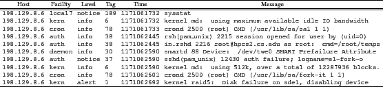
Syslog is primarily responsible for managing the log file while the message content is largely created by the application. As seen in figure 1, messages do have a specific format consisting of the six fields. In this example, the host field is the IP of the machine sending the message (since one syslog instance may serve multiple computers). The facility field is the source of the message, for example kernel or user space. The level indicates the severity of the message, which ranges from general to critical. The tag field is a positive integer that represents the facility and level fields where lower tag values represent more critical messages. For example in figure 1, a disk failure has a tag value of 1 while the execution of a command (first message) has a tag value of 189. Since this value is the combination of the facility and level, it does not reflect the actual message content. For example in figure 1, the tag value 38 occurs twice although the message content is different.
The time field is the time the message was recorded by the syslog facility. Finally, the message is the text portion of the entry that describes the event that has occurred. The message is created by the application and is a free-form field. This makes analysis more difficult requiring complex natural-language parsers. However, recent research has been successful in associating certain words that appear in the log file messages with critical future events [11].
 |
Although a wide variety of log file messages exist, Self-Monitoring Analysis and Reporting Technology (SMART) messages are of interest since they provide information specific to disk drive health. SMART boards are becoming a standard component of ATA and SCSI hard disks. SMART disk drives internally monitor their health and warn of impending hard disk drive problems. In many cases, the disk itself provides advance warning that something is wrong long before actual disk failure. Most implementations of SMART also allow administrators to perform self-tests and monitor performance and reliability attributes.
The smartd daemon regularly monitors the disk's SMART data for signs of problems. When smartd is started, it registers the system's disks then checks their status every 30 minutes for attributes indicating failure. If there is a failing health status or an increased number of errors or failed self-tests, the daemon sends this information to the system log file. Pinheiro et al. found that while some SMART parameters do correlate with drive failure, these messages alone are insufficient for prediction [9].
As described in the introduction, a Support Vector Machine (SVM) is a supervised machine-learning method that can be used for binary classification: associating a non-labeled sample to one class or another. Given a set of labeled training data (features) the SVM finds the best plane that separates the two classes. If the data is not linearly separable, then it is possible to translate the data into a higher-dimensional space to find a separator, referred to as the kernel-trick. Once the plane has been found, the SVM can associate new non-label data to a specific class. Furthermore SVMs allow the inspection of weight functions, making it possible to identify which features are most responsible for classification.
The SVM can be used for predicting system failure by concluding
that a series of messages are or are not associated with failure
in the future. Let ![]() represent a time-ordered set of log file
messages for a single computer. Therefore, the sequence of
messages that appear in
represent a time-ordered set of log file
messages for a single computer. Therefore, the sequence of
messages that appear in ![]() form a time-series representation of
events that occurred. For this paper let each message in
form a time-series representation of
events that occurred. For this paper let each message in ![]() be
represented by its tag value, which provides an indication of
message criticality. For the messages given in figure
1, the set
be
represented by its tag value, which provides an indication of
message criticality. For the messages given in figure
1, the set ![]() would be
would be
![]() .
.
Using ![]() it is possible to collect various aggregate features,
such as the frequency of tag values. For the messages in figure
1: the tags 189, 30, 37, and 1 occur once; and the
tags 78, 38, and 6 occur twice. This forms a vector describing
it is possible to collect various aggregate features,
such as the frequency of tag values. For the messages in figure
1: the tags 189, 30, 37, and 1 occur once; and the
tags 78, 38, and 6 occur twice. This forms a vector describing ![]() as (1:1, 6:2, 30:1, 37:1, 38:2, 78:2, 189:1), where each value is
the
tag:count. This vector can then be used to
classify
as (1:1, 6:2, 30:1, 37:1, 38:2, 78:2, 189:1), where each value is
the
tag:count. This vector can then be used to
classify ![]() as belonging to a fail or non-fail system.
as belonging to a fail or non-fail system.
The frequency of tag values in ![]() can help predict system events,
however, additional valuable information is found in the sequence
of messages. Identifying certain sequences of
messages, represented by tag values, that are a prelude to a certain
system events is one specific example. The spectrum kernel representation of the log
messages will provide this ability for SVM classifiers.
can help predict system events,
however, additional valuable information is found in the sequence
of messages. Identifying certain sequences of
messages, represented by tag values, that are a prelude to a certain
system events is one specific example. The spectrum kernel representation of the log
messages will provide this ability for SVM classifiers.
The spectrum kernel representation of data was developed by Leslie
et al. for determining protein sequence similarity
[6]. This representation used a ![]() -length sequence of
amino acids as a feature for proteins. The proteins representation
was then the number of times sequences occurred as a
-length sequence of
amino acids as a feature for proteins. The proteins representation
was then the number of times sequences occurred as a ![]() -length
window is passed over the sequence of amino acids. The
spectrum-kernel representation has also been used for network
connection classification [13] and intrusion
detection systems [2]. In this paper we apply this
approach to sequences of system log messages, specifically the tag
values.
-length
window is passed over the sequence of amino acids. The
spectrum-kernel representation has also been used for network
connection classification [13] and intrusion
detection systems [2]. In this paper we apply this
approach to sequences of system log messages, specifically the tag
values.
The spectrum representation of ![]() will consist of the frequency
of the different possible
will consist of the frequency
of the different possible ![]() -length sequences. The number of
possible sequences is
-length sequences. The number of
possible sequences is ![]() , where
, where ![]() is the number of
different tag values. Given the finite amount of memory available
to store information, limiting either the window size
is the number of
different tag values. Given the finite amount of memory available
to store information, limiting either the window size ![]() and/or
the tag range
and/or
the tag range ![]() may be necessary. For example, assume there are
65536 possible tag values and the window length is 5, then there
are
may be necessary. For example, assume there are
65536 possible tag values and the window length is 5, then there
are
![]() possible tag sequences. Therefore,
limiting the tag range allows the consideration of longer
sequences and vice versa.
possible tag sequences. Therefore,
limiting the tag range allows the consideration of longer
sequences and vice versa.
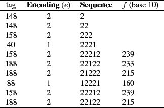
Assume ![]() consists of the 10 tag values given in figure
2. Let the window size be 5, which is also the
sequence length,
consists of the 10 tag values given in figure
2. Let the window size be 5, which is also the
sequence length, ![]() . Furthermore, associate each tag with one of
three levels, high (tag
. Furthermore, associate each tag with one of
three levels, high (tag ![]() ), medium
(
), medium
(![]() tag
tag![]() ), low (tag
), low (tag![]() ). In this example
). In this example ![]() is
three which results in 243 possible sequences, substantially lower
than if no levels are used. Let the level representation of a tag,
or encoding, be denoted as
is
three which results in 243 possible sequences, substantially lower
than if no levels are used. Let the level representation of a tag,
or encoding, be denoted as ![]() . Assign the high level tag the
encoding value 0, the medium level 1, and low level 2.
. Assign the high level tag the
encoding value 0, the medium level 1, and low level 2.
To find the sequences in ![]() , pass a
, pass a ![]() -length window over
-length window over
![]() and record the sequence occurrences. For example
consider again the messages in figure 2. The
sequence
and record the sequence occurrences. For example
consider again the messages in figure 2. The
sequence ![]() (which corresponds to three low level
messages, one medium message, followed by one low level message)
occurs twice. Similarly, the the sequence
(which corresponds to three low level
messages, one medium message, followed by one low level message)
occurs twice. Similarly, the the sequence ![]() twice, while
the sequences
twice, while
the sequences ![]() , and
, and ![]() occur only once. All
other possible sequences do not occur in this example.
occur only once. All
other possible sequences do not occur in this example.
Let each sequence be represented by a unique value, ![]() . For
example, the feature value 239 identifies the sequence
. For
example, the feature value 239 identifies the sequence ![]() .
As described in [13], this can be done using a
process that only requires storing the previous feature value
.
As described in [13], this can be done using a
process that only requires storing the previous feature value ![]() and the new tag number encoding. The
and the new tag number encoding. The ![]() feature value can be
determined using the
feature value can be
determined using the ![]() feature and tag number encoding, the
feature value for the
feature and tag number encoding, the
feature value for the ![]() feature is
feature is
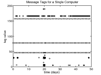
The SVM approach to predicting system events was evaluated experimentally using actual system log files. The log files were collected over approximately 24 months from a 1024 node Linux-based compute cluster. Each computer was similarly configured and consisted of multiple processors and disks. The system event predicted was hard disk failure, since it is easy to identify in the log file, for example the last message in figure 1 is a disk failure.
The log files contained over 120 disk failure events. For a single computer it is possible to have multiple disk failures within a relatively short period of time, since each computer has multiple disks. In this case only disk failures that were separated by at least one day were considered. This was done to eliminate any messages that may have been due the previous failure. As a result, only 100 of the 120 failures were usable for the experiments.
 |
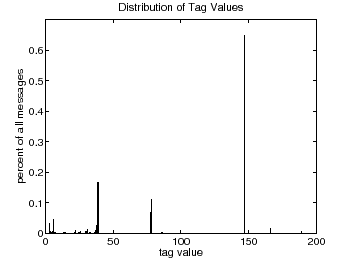
The log files averaged 3.24 messages per hour per system. Therefore each machine averaged approximately 78 messages per day. The distribution of tag values are given in figure 4. There were 61 unique tag values, ranging from 0 (the most critical message) to 189 (least important message). As seen in the histogram certain tag values appear more frequently, a fact that we use to determine the appropriate tag ranges as described in the previous section.
A set of 1200 messages (approximately 15 days of data) was
collected from systems that did and did not experience a disk
drive failure. For computers that experienced a failure, the last
message of the 1200 is a disk failure message. Starting at the
first message in the set, a sub-set of messages, ![]() , was used to
make a prediction. The length of
, was used to
make a prediction. The length of ![]() equaled 400, 600, 800, 1000
or 1100 messages. Therefore when
equaled 400, 600, 800, 1000
or 1100 messages. Therefore when ![]() equals 1000 messages, only
200 messages remain before the failure event. Larger values of
equals 1000 messages, only
200 messages remain before the failure event. Larger values of ![]() should result in better predictions since more data is available.
should result in better predictions since more data is available.
Hold-out was used to partition the samples, where half of the disk failure sets are randomly selected for training and the other half is used for testing. An equal number of fail and non-fail sets were used per experiment. Hold-out was repeated 100 times per experiment and the average performance was recorded.
As described in the introduction, the objective of event prediction is to accurately predict disk failure as far as possible in the future. Given a binary classifier and an input, four outcomes are possible [3]. Assume the input is in the positive class. If the classifier predicts positive then the outcome is a true positive. If the classifier predicts negative then the outcome is a false negative. If the input is negative and the outcome is negative, then it is a true negative. If the input is negative and the outcome is positive, then it is a false positive. For this paper let the positive class represent drives that do not fail. Therefore a false positive is a drive predicted not to fail but does, in contrast a false negative is a drive predicted to fail but does not.
The percent accuracy, precision, and recall was recorded for each experiment. Accuracy is the total number of correct predictions (fail and non-fail) divided by the total number of inputs. Precision is the number of true positive divided by the number of true positives and false positives. Recall is the number of true positives divided by the number of positive inputs. A predictor with a high precision has fewer false positive errors (predicted good but actually fails), while a predictor with a high recall has fewer false negative errors (predicted to fail but is good).
Another measure of classifier performance is the Receiver
Operating Characteristics (ROC) curve [3]. As seen in
figure 5(b), false positive rate is plotted against the
true positive rate. The graph shows the trade-off benefits (true
positives) and costs (false positives). For example, the point ![]() represents a classifier that never generates a positive
classification. This classifier would not have any false positives
but would not have any true positives either. The opposite is
true for the point
represents a classifier that never generates a positive
classification. This classifier would not have any false positives
but would not have any true positives either. The opposite is
true for the point ![]() , which is a classifier that never
generate a negative classification. The point
, which is a classifier that never
generate a negative classification. The point ![]() represents
a perfect classifier since the true positive rate is maximized and
the false positive rate is minimized. Therefore, an ROC curve that
is close to the top left-hand corner of the graph is considered a
good classifier. In contrast, the line between points
represents
a perfect classifier since the true positive rate is maximized and
the false positive rate is minimized. Therefore, an ROC curve that
is close to the top left-hand corner of the graph is considered a
good classifier. In contrast, the line between points ![]() and
and
![]() represents a random classification outcome for any given
input.
represents a random classification outcome for any given
input.
Finally, the Area Under the Curve (AUC) for an ROC is often used to measure classifier performance. The area for the perfect classifier is 1 while a random classifier is 0.5 (area below the diagonal), therefore a classifier should have an AUC between 1 and 0.5.
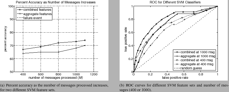 |
Two different SVM classifiers were used for each experiment, differing only in the features used. One SVM used only those aggregate features which occured in the logs, which is similar to the approach taken by [8]. Since only 190 tag values occurred, only 190 features are possible. The second classifier used aggregate and a spectrum representation of the messages, will be referred to a combined features. The spectrum representation considered sequences of 5 messages. Tag values were associated with one of 19 ranges. The range values were determined from the tag histogram and group the most popular tag values together. As a result, 2,476,289 features are possible.
As previously described, given 1200 messages, the first 400, 600, 1000, and 1100 messages were used to make a prediction. Figures 5 and 6 show the performance as the messages are processed. As seen in figure 5(a), the accuracy of the aggregate features ranged from 64% to 70% as the number of messages increased from 400 to 1100. These values are commensurate with other SVM based approaches. The increase in accuracy is expected since more messages provide a more information to make a prediction. The precision and recall percentages were similar to the accuracy.
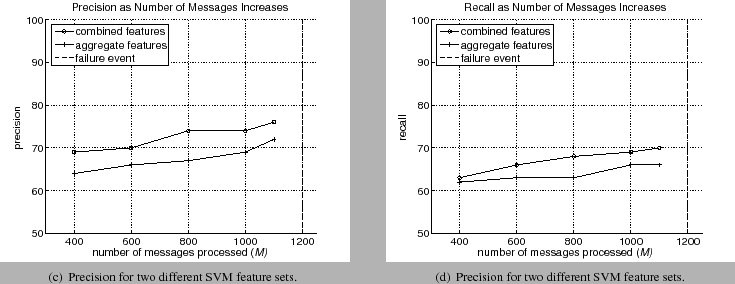 |
The performance of the SVM using the combined features (aggregate and spectrum representations) was higher than the SVM using only aggregate features. The accuracy ranged from 67% using only 400 messages to 73% using 1000 messages and 74% using 1100 messages. Therefore at 200 messages before the failure event (approximately 60 hours before failure), the SVM can predict failure with 73%. The precision and recall had similar values. This increase in performance indicated the addition of sequence information can improve performance.
The ROC curves, given in figure 5(b), show the same performance benefits. At 400 messages the combined features has an advantage over aggregate features only. The AUC was 0.72 for the combined features and 0.65 for the aggregate features. Aggregate features are only slightly better than a random classification. However when the number of messages processed is 1100, there is an increase in performance. The AUC is 0.79 for the combined features and only 0.72 for the aggregate. The small linear portion of the combined feature ROC curves indicate classifier generated false positives for certain sets of messages. Regardless, the combined features consistently performed better.
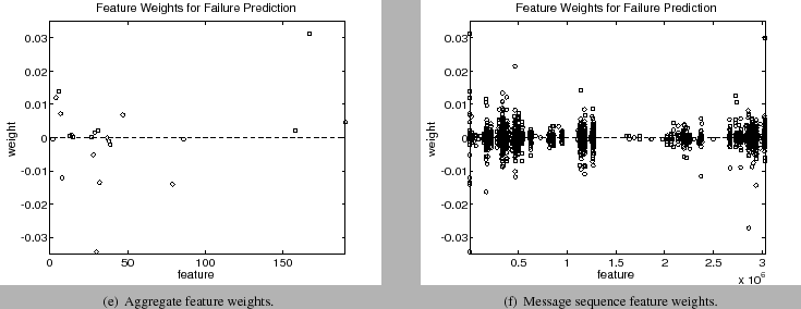
The importance of certain features can be considered by analyzing the feature weights and is possible since the linear kernel was used. Figure 7 shows the weights of the aggregate and sequence features. Of the 2,476,289 possible combined features, only 2,251 had a non-zero weight when used for failure classification. A positive weight indicates the feature is useful for classifying a disk failure, while a negative weight is useful for classifying a non-failure. Larger values (positive or negative) indicate a better feature.
As seen in figure 7(a), only 22 aggregate features were used for classification. Of these features 9 were for non-failure and 13 were for disk failure. The remaining 2,232 features, seen in figure 7(b) represented the occurrence of different message sequences. As noted from the experimental results, the message sequences play an important role in failure prediction.
 |
Computer system failures result in the loss of productivity and increased operation cost [7]. Better management of computer resources, applications, and services is possible given accurate predictions of system failures.
Log files typically contain useful information about system failures. These files record the history of the system's state which provides administrators information to determine the causes of critical events. Although log file analysis has been primarily performed after an event has occurred, increasingly this information is being used to predict events.
This paper introduced a new system failure prediction method using
Support Vector Machines (SVM) based on the information contained
in log files. The proposed approach takes advantage of the
sequential nature of log messages and determines which sequence
of messages are precursors to failure. Messages were represented
using the tag value, which offers an indication of message
criticality. A spectrum kernel representation of the tag values
was then used to describe a set of messages, which measures the
frequency of ![]() -length message sequences. Experimental results
using log files from a large 1024 node Linux-based compute cluster
indicate the the spectrum-representation of messages combined with
a SVM classifier can achieve an accuracy of 73% and a two day
lead (amount of time before the event). Results also show that
more log messages consistently provide better predictions.
-length message sequences. Experimental results
using log files from a large 1024 node Linux-based compute cluster
indicate the the spectrum-representation of messages combined with
a SVM classifier can achieve an accuracy of 73% and a two day
lead (amount of time before the event). Results also show that
more log messages consistently provide better predictions.
Although the results indicate the spectrum-representation has promise, there are several open questions. Additional features, such as message interarrival times [8], should be considered. The performance of the system could also be improved by leveraging the message content, instead of solely relying on the tag value. For example, the information provided by SMART messages could be used as a feature. However adding more message information must be balanced with the sequence length, since the number of features grows exponentially. Finally, more research is needed to study the impact of message diversity, which can be the result of machine purpose and log generation rates.
This document was generated using the LaTeX2HTML translator Version 2008 (1.71)
Copyright © 1993, 1994, 1995, 1996,
Nikos Drakos,
Computer Based Learning Unit, University of Leeds.
Copyright © 1997, 1998, 1999,
Ross Moore,
Mathematics Department, Macquarie University, Sydney.
The command line arguments were:
latex2html -split 0 -show_section_numbers -local_icons -no_navigation wasl08f.tex
The translation was initiated by Errin Fulp on 2008-11-10