
Hunting for problems with Artemis
Gabriela F. Creţu-Ciocârlie, Mihai Budiu and Moises Goldszmidt
gcretu@cs.columbia.edu,
{mbudiu,moises}@microsoft.com
Microsoft Research, Silicon Valley
Artemis is a modular application designed for analyzing and troubleshooting the performance of large clusters running datacenter services. Artemis is composed of four modules: (1) distributed log collection and data extraction, (2) a database storing the extracted data, (3) an interactive visualization tool for exploring the data, and (4) a plug-in interface (and a set of sample plug-ins) allowing users to implement data analysis tools including (a) the extraction and construction of new features from the basic measurements collected, and (b) the implementation and invocation of statistical and machine learning algorithms and tools. In this paper we describe each of these components and then we illustrate the power of the plug-in architecture by presenting a case-study using Artemis to analyze a Dryad application running on a 240-machine cluster.
The computer industry is in the midst of a new revolution: the emergence of cloud computing. Many players in the industry are building cloud-based services using large clusters of commodity PCs.
Key to the effectiveness of cluster computing is reduced resource management cost. However, writing distributed software systems for large clusters, debugging, optimizing performance, monitoring, repairing, provisioning, and upgrading are difficult tasks. One of the main tools used by software developers for cluster services is abundant logging information. Since the use of debuggers on live server-side systems is most often impossible, logging is the tool of choice for understanding large-scale system behavior. Thus even live deployed systems contain copious amounts of logging.
As a consequence, an important part of meeting the performance and dependability goals of clusters is the management and analysis of distributed logs. Understanding performance frequently requires the aggregation of log information across the machines in the cluster. Debugging correctness problems requires the correlation of log information, to infer system interactions. Automated analysis using statistical machine learning algorithms requires performing tasks such as feature extraction and visualization.
In this paper we describe Artemis, an application for the analysis of large-scale distributed logs, that incorporates all the elements mentioned above. Artemis has been designed to be modular, separating data collection from data analysis, and separating application-specific parts[1] from generic application-independent parts. We show how the flexibility of Artemis allows us to customize it for the domain of distributed Dryad applications (Dryad is described briefly in Section 3). In Section 5 we use this customized instance of Artemis for debugging a Dryad application running on a 240-machine cluster. We have also used Artemis to explore datasets produced by other distributed applications, such as telemetry performance data for the Windows operating system and performance measurements from a data center providing enterprise services.
As an application focused on the analysis of distributed logs, Artemis presents the following unique combination of characteristics:
· Artemis integrates in a single tool all the important tasks required for log analysis: collection, storage, visualization, analysis; it is designed to be a one-stop shop for the programmer attempting to understand the performance of a distributed application. The system architecture integrating all of these pieces is the subject of Section 4.
· Artemis is modular and extensible in several dimensions:
- Artemis can manipulate multiple data sources and data types. Our current data sources include log (text) files, performance counters data (stored in comma-separated files with headers), XML data sources, and binary (encoded) dumps from a variety of sources (application and system-level). We discuss data collection in Section 4.1.
- Artemis performs both generic and user-defined data analyses. A plug-in mechanism allows the data analyst to write (or invoke) additional domain-specific analyses. In this paper we include a description of several plug-ins we wrote for the analysis of Dryad jobs: “machine usage”, “job critical path”, and “network utilization”.
· Artemis is built around a Graphical User Interface (GUI), keeping the human in the data analysis loop. The GUI, described in Section 4.3 enables the analyst to quickly navigate data visualizing correlations and trends, and also to define interactively the features used for more sophisticated machine-learning data analyses. The visualization tool provides two basic primitives: histograms and time series.
There is a lot of prior work in (distributed) log collection, log visualization and log data analysis. We believe that Artemis is unique in integrating all these activities into a single tool in a generic (application-independent) and extensible architecture. We enumerate here only papers related to distributed log analysis and highlight the differences with Artemis.
Pablo [10] is an early system with many similar goals, but a very different realization.
LogSurfer and LoGS [8,9] focus on closing the feed-back loop, using on-line corrective actions when faults are detected in the system.
NetLogger [2] combines data from network, host and application events. It contains four components: an API for generating application-level events, a set of tools for collecting and sorting log, a set of host and network monitoring tools and a front-end visualization tool. It requires the analyzed application to use the special logging libraries.
A lot of research has been dedicated to datamining distributed systems logs (MapReduce, Hadoop, and grid computing systems). Recent examples include [5,6,12,14]. The work in [5,14,12] focuses on taking advantage of syntactic features in the logs. The work in [6] is built around machine learning techniques for performance debugging, yet it is not integrated with visualization, feature extraction, and it is not easily extendable (with new algorithms) as Artemis is.
As discussed in the introduction, while Artemis can then be used for analyzing the performance of various distributed computing applications, in this paper we focus on the use of Artemis for analyzing Dryad-based distributed applications[2]. Dryad [3] is middleware for building data-parallel distributed batch applications. The structure of a Dryad application (called a Dryad job) is depicted in Figure 1. A job is composed from a set of stages; each stage is composed of an arbitrary number of replicas of a vertex (each operating on a different data partition). The edges of the graph are point-to-point communication channels. The job graph is required to be acyclic. Communication channels are finite sequences of arbitrary data items. In general each vertex corresponds to a single process, but several vertices connected with shared-memory channels can be run as separate threads in the same process.
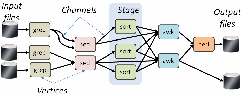
Figure 1: structure of a Dryad job.
This model is simple and powerful. Despite the fact that the Dryad runtime is unaware of the semantics of the vertices (i.e., the vertices can run arbitrary binaries), the Dryad runtime can provide a great deal of functionality: generating the job graph, scheduling the processes on the available machines, handling transient failures in the cluster, collecting performance metrics, visualizing the job, invoking user-defined policies and dynamically updating the job graph in response to these policy decisions.
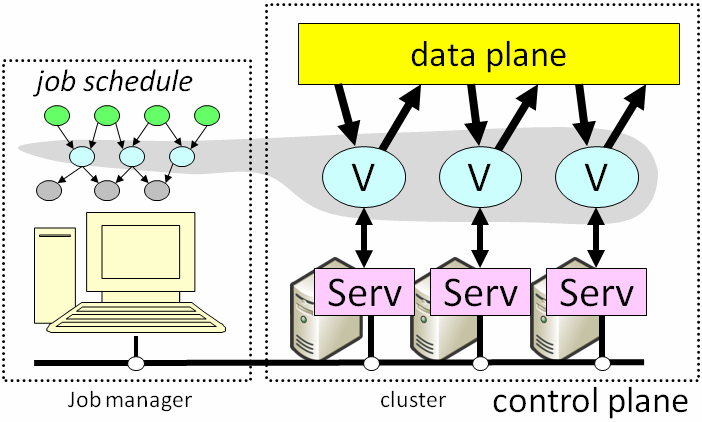
Figure 2: Dryad system architecture.
Figure 2 shows schematically how Dryad is implemented. Each Dryad job is supervised by a centralized job manager process. The job manager uses a small set of cluster services to control the execution of the vertices on the cluster. The minimal set of services required for Dryad’s operation include a name service and a remote execution service. All these components (JM, services, vertices) produce logging information.
Figure 3 shows the structure of the Artemis distributed log-analysis toolkit. Artemis attempts to cleanly separate the application-specific parts from the application-independent parts. Artemis can be adapted for analyzing a new distributed application by replacing or modifying the application-specific parts.
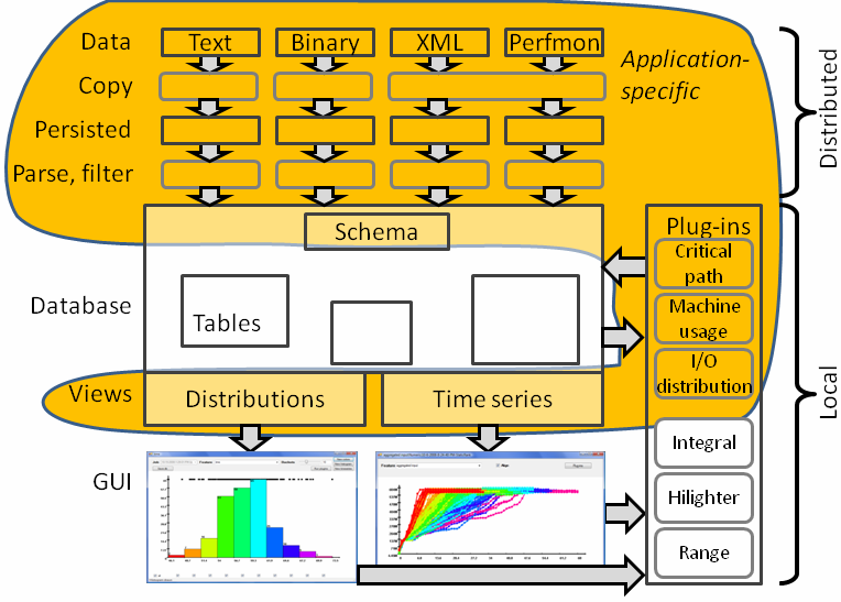
Figure 3: Artemis architecture. The application-specific parts have been highlighted.
The four main components of Artemis are:
1. Log collection, persistence, filtering and summarization. These are application-specific; their role is to collect log data about the application and to translate it to a uniform format.
2. Data storage. The collected data is stored using a generic database. Only the schema is application specific.
3. Data visualization. Interaction with the data is done by using an entirely generic GUI, which can display histograms and time series data. The GUI is coupled to the database using a pair of (application-specific) views: one providing data for the histograms and the other providing data for the time-series.
4. Data analysis is implemented using a plug-in architecture. A plug-in is an object implementing a specified .Net interface; the inputs and outputs of plug-ins are views of the database. Some plug-ins are generic (e.g., computing the area under a curve), while other are application-specific (e.g., computing the critical path of a Dryad job). The data generated by running a plug-in is merged back into the database, and thus can be visualized with the GUI or used by other plug-ins.
We proceed to describe each of these components.
The data-collection front-end for analyzing Dryad jobs aggregates data from the following sources: (a) the job manager logs, (b) the logs of the vertices, generated by the Dryad runtime library (linked to each vertex), (c) logs from the remote execution cluster services, which fork vertices and collect statistics about them, (d) performance counters from the Windows performance monitoring service (Perfmon) and (e) logs from the cluster name server describing the cluster network topology. Some of these logs are text files (a, b, d above), while other are XML (e) or binary-encoded (c). It is straightforward to add additional sources of information; for example, we plan to add SNMP logs from cluster routers.
A single Dryad job composed of tens of thousands of processes and running on a large cluster for tens of minutes can emit in excess of 1TB of logs. Each Dryad vertex process runs in a sandbox, having a private home directory where the vertex maintains its working space, and where the vertex dumps logs. Each vertex produces around 1 MB/s/process. Following the completion of a Dryad job, the cluster-level job scheduler garbage-collects the sandboxes of the job vertices after a configurable time interval.
We have built an additional application-specific GUI front-end for interfacing Artemis with the Dryad cluster scheduler. This GUI enables the data analyst to browse the jobs residing on the cluster and to choose which ones to copy and analyze. Artemis first parses the job manager logs which contain global per-job information, including pointers to the location of all the vertex logs. This information is used to prepare the input for a distributed DryadLINQ [15] computation, which locates, copies, reads, parses, and summarizes all the distributed data sources which reside on the machines in the cluster[3].
Using DryadLINQ enables the Artemis data collection to take advantage of the parallelism available in the very cluster under study for the data-intensive parts of the analysis. The DryadLINQ computation spawns a vertex on each machine which contains interesting logs. On our 240-machine cluster filtering several hundred gigabytes of log data requires just a couple of minutes of wall-clock time.
The cluster services and the performance counter collection tasks are running and logging continuously on each machine in the cluster; in contrast, a Dryad vertex uses a machine for a bounded time. The Artemis log collector extracts only the relevant portions of the service logs for each machine. Data extraction involves, in essence, performing a giant distributed join.
The information extracted from vertex logs includes the I/O rate for each Dryad channel. The performance counters include over 80 entries describing global (per-machine) and local (per-process) measurements (e.g., virtual memory usage, I/O rate, garbage collections, processor utilization, etc). The counters include information about the .NET runtime. The remote execution daemons provide statistics about all the Dryad channels.
The filtered data from all these sources is extracted and aggregated in a database accessible from the local workstation. In principle any relational engine could be used, and we plan to use a commercial database in the future.
The most important part of the database is the data schema. The schema is generated by the data collection process. The schema can categorize each table column as one of: numerical data (e.g., CPU utilization), category (e.g., machine name), string (e.g., channel URI), or timestamp or time offset (e.g., time when record was collected). This approach is similar the one used by the Polaris [13] data visualization tool.
The data visualization part of Artemis is completely generic (i.e., it is not tied to the application), and is not tied to the data semantics (the only data semantics is conveyed by the schema). We have focused on displaying two types of magnitudes:
· Scalar-valued measurements, which can be of type either numeric or category (e.g., starting time, total I/O, machine where a vertex has run, number of garbage collections);
· Time series data (e.g., I/O in each 2 second interval, CPU utilization in each interval, etc). By definition, a time-series is composed of data items tagged with timestamps.
In order to interface the database with the visualization a domain expert must create two application-specific database views. The first view is a relation containing all database columns that contain scalar data; the “primary key” of this table is the main entity which is analyzed (in our case study the key is the ID of a Dryad job process).
The second view is a relation that must contain at least two columns: one column is a foreign key pointing to the primary key of the first view; the second column is a timestamp (absolute or relative). The other columns of this view contain time-series data. In our case, all performance data collected by Perfmon maps directly into this view.
The data from the first view (scalar data) is browsed and displayed using histograms and distributions (shown in Figure 4); and the data from the second view is displayed with line-plots (shown in Figure 6).
The user can choose using drop-down boxes the metrics to display (in essence performing a relational algebra projection of the view on a selected column), and the number of buckets of the histogram. In Figure 4 the user has displayed the running time of the Dryad job processes in a particular stage, and she has used a histogram with 10 buckets; only the first 4 and the last buckets contain any elements. Once a histogram has been displayed, each primary key value is associated with a color (the color of the bucket of the histogram). For example, the leftmost (fastest) 45 processes become red, and the next 157 processes become orange, while the lone outlier at the right is magenta.
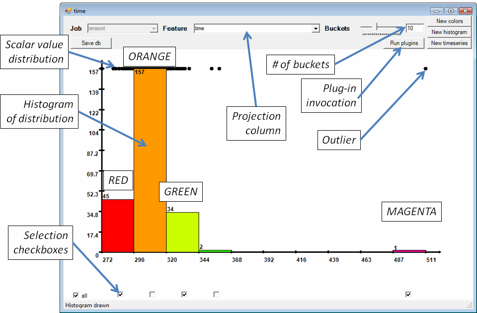
Figure 4: Displaying a set of scalar values using a histogram. The horizontal axis is the value being histogramed, in this case running time.
The GUI preserves these colors across different displays; Figures 5, 6, 10 and 11 use the same color assignment. For example, in Figure 5 we display the distribution and histogram of another scalar value, the peak number of page faults (measured across 15-second intervals). For each process the same color as in Figure 4 is used. This makes it easy for the user to identify for example, whether misbehaved instances are also outliers with respect to other metrics. In Figure 5 below we note that the outlier from Figure 4 continues to be an outlier with respect to the “peak number of page faults”. Each histogram bucket can be “selected” with a checkbox; only the data from the selected buckets is used in further analyses (in essence performing a relational algebra select operation visually).
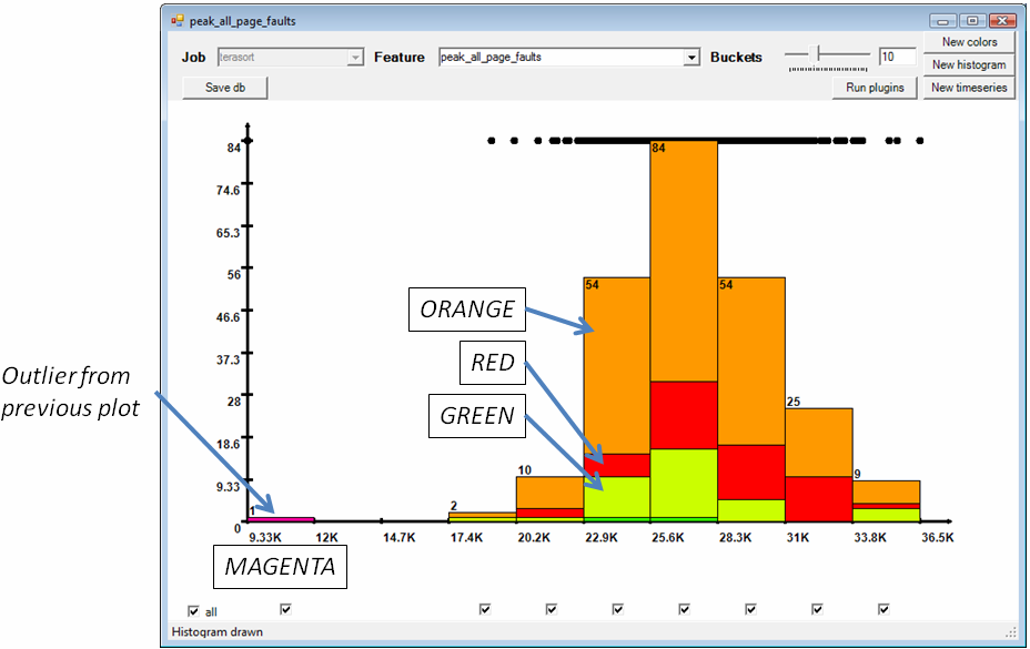
Figure 5: Peak number of page faults; this histogram uses the same color coding as in Figure 4.
The second type of data that can be visualized is the time-series. Time series are drawn with lines using the colors inherited from a histogram (using the foreign key). For example, in Figure 6 we display the “disk read rate” (number of bytes read from disk in each 15-second interval) for 3 selected buckets: red, green and magenta. We can see that with respect to this metric the magenta process is not an outlier, since its line is right in the middle of the pack.
Multiple time series can be aligned (to start all at the same time) or unaligned (they are displayed in absolute time). Figure 6 is an aligned view, while Figure 8 is unaligned.
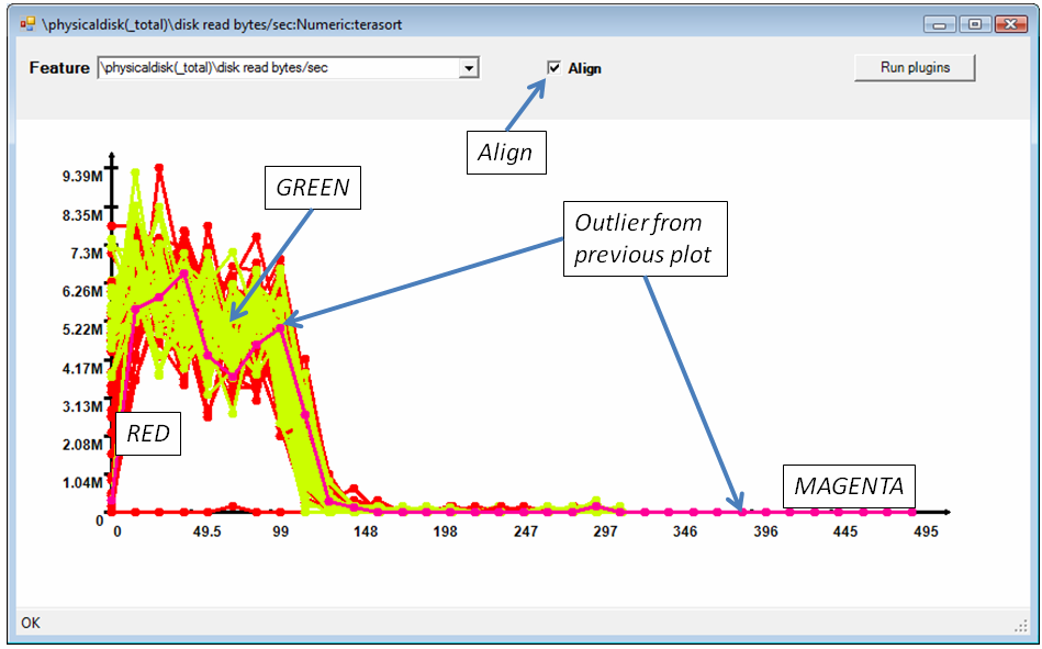
Figure 6: Time series of the disk I/O rate for selected processes. The horizontal axis is always time when displaying a time-series, while the vertical axis is the magnitude being plotted (disk rate).
The displays allow the user to click on points or buckets or to use a rubber-band to select data. The GUI identifies the selected data using a tabular display shown in Figure 7. The tabular display can be used to make further projections and selections, and to export data directly to Excel. For example, using the tabular display we can find out which one is the outlier process from Figure 4.
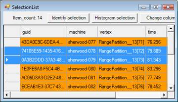
Figure 7: Data from plots displayed in a tabular view.
We can interpret the data displayed by a GUI window as (yet another) relational view of the data (obtained from the projection of the input view on selected columns followed by selection of the chosen buckets). This is important because the displayed data can be fed to plug-ins for further analysis.
Each GUI window contains a “Run plug-ins” button which can be used to invoke computations on the current data view.
Data analysis in Artemis is performed with plug-ins. The plug-ins are used for (1) computing meaningful features from the data, for driving the statistical analyses; (2) for invoking statistical analysis and machine learning packages, and (3) for performing application-specific data analyses, including running “scripts” invoking other plug-ins. We give examples of each of these analyses for the case of Dryad jobs.
We provide a library of generic plug-ins for computing simple data transformations which can be composed to compute new metrics from existing data. For time-series data we have min, max, range, average, integral, derivative, anti-derivative, and variance plug-ins. Some of these plug-ins generate new time-series (e.g., derivative), while other generate scalar data (e.g., average). Since the GUI has no knowledge of data semantics, the data analyst has to use application-specific knowledge to decide which of these transformations are meaningful (e.g., you can integrate CPU time to obtain work, but you cannot integrate the machine-usage time-series described in Section 4.4.3.)
The plug-ins can be invoked either interactively from the GUI or as batch computations from other plug-ins. The data computed by the plug-ins is merged into the database for immediate visualization or further analyses.
When analyzing Dryad jobs we combine the scalar metrics extracted from the logs with the computed features to generate new features for each Dryad process; these features can be used by the statistical machine learning plug-ins. We chose not to prune the collected metrics, but instead we use automated statistical approaches [1] to decide which features are important.
Currently we have implemented plug-ins interfacing Artemis with two off-the-shelf statistics packages (developed at Microsoft): data clustering and statistical pattern classification and feature selection. The plug-ins write data to files as expected by each analysis package and then invoke external processes to perform the analysis. One such plug-in is written in roughly 100 lines of code, so we expect it would be easy to interface Artemis with other statistics packages.
The clustering analysis attempts to uncover differences in performance among the analyzed entities (e.g., Dryad processes) and to determine which of the available features correlate with those differences. When applied in the context of Dryad, this analysis relies on the assumption that all vertices in a stage exhibit similar behavior. The differences between vertices in a stage provide evidence for either: a) faulty hardware, b) bad data distribution, c) uneven data sizes, and d) interference with other processes running on the same machine. The clustering analysis uses a standard k-means algorithm with automated model selection (the number of clusters[4]). The model selection is done by evaluating the change in distortion when increasing the number of clusters. The clustering algorithm groups vertices according to their similarity in performance while pointing to outliers.
The pattern classification analysis is directed at explaining differences in the performance of the vertices belonging to different clusters. The analysis automatically induces a model that discriminates between the vertices according to their cluster. The analysis uses logistic regression with L1-regularization [4]. This is an effective method for feature selection in classification, especially when the number of features is comparable to the number of samples [4]. We rely on a tool called HiLighter [1] which was designed for diagnosing performance problems in systems ranging from enterprise cloud computing to test-bed software debugging.
The most powerful kinds of Artemis plug-ins have access to the entire measurement database. These plug-ins can implement complex data analyses by joining information from multiple tables in an application-specific way. We give three examples of plug-ins we have developed specifically for analyzing Dryad jobs.
a) Machine usage. This plug-in computes machine usage for an entire job and represents it using time-series data, enabling visualization with the existing GUI. For each process it creates a time series with four points, corresponding to the essential state-transitions of the process: “ready to run”, “scheduled to run”, “starts running”, “terminated”. The x axis is time, while the y axis is the home machine of each process. Figure 8 shows the machine usage for the distributed sorting application that we discuss in Section 5.

Figure 8: Machine usage data displayed as a time-series.
The machine usage plug-in enables the fast visual identification of which stages carry the weight of the computation (i.e. take the longest time to finish), which are the longer running vertices, and where are the scheduling bottlenecks. The execution shown in Figure 8 has poor cluster utilization due to some late-scheduled vertices (all stages in this application are blocking, requiring the previous stage to complete before starting).
b) Critical path. The critical path shows the longest chain of dependent processes in a Dryad job graph execution. When overlaid with the machine usage plot, the critical path shows where the bottleneck of a particular computation is.
c) Network utilization. This plug-in combines several database tables to compute the network traffic distribution. It uses the cluster topology database (describing machine assignment to racks) and the description of all job channels (input URI, destination process, machine mapping of processes) to determine how the job data traffic is distributed on the network.
We have used Artemis to diagnose problems for several DryadLINQ computations running in a research cluster comprising 240 machines. The machines are all running Dryad; they all have 4 CPU cores, 4 striped disks and 16 GB of memory. In this section we choose a representative Dryad application, written in DryadLINQ: distributed sorting. The DryadLINQ compiler generates a plan comprised of 4 stages, shown in Figure 9. The input is stored in a 1Tb file partitioned into 240 pieces.
The first stage of the application reads the whole file in parallel using 240 vertices and samples uniformly from the input. The second stage aggregates the samples and computes the distribution of the sampled input. It also computes the boundaries of 240 equal-sized buckets which will be used to redistribute the input. The third stage reads the whole input again and performs a hash-distribution using the buckets computed by stage 2. Finally, each vertex in the fourth stage performs an in-memory multi-threaded sort and writes the output to its local disk.
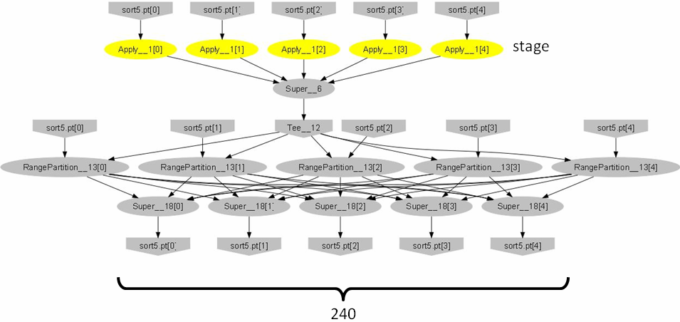
Figure 9: Distributed sorting: an application analyzed using Artemis.
The machine usage during one execution of this application is in Figure 8. Stage 2 (histogram) is extremely fast and barely visible. All the other figures in this paper show just data related to the sorting stage[5].
In Figure 8 we notice two anomalies in the sorting stage: one vertex starts much later than the other ones, and the running time of one vertex is much longer. The late vertex is due to scheduling conflicts on the cluster: this vertex and another one have been run sequentially on the same machine. This information tells us that even in the absence of the long-running outlier this stage would have taken a long time to complete.
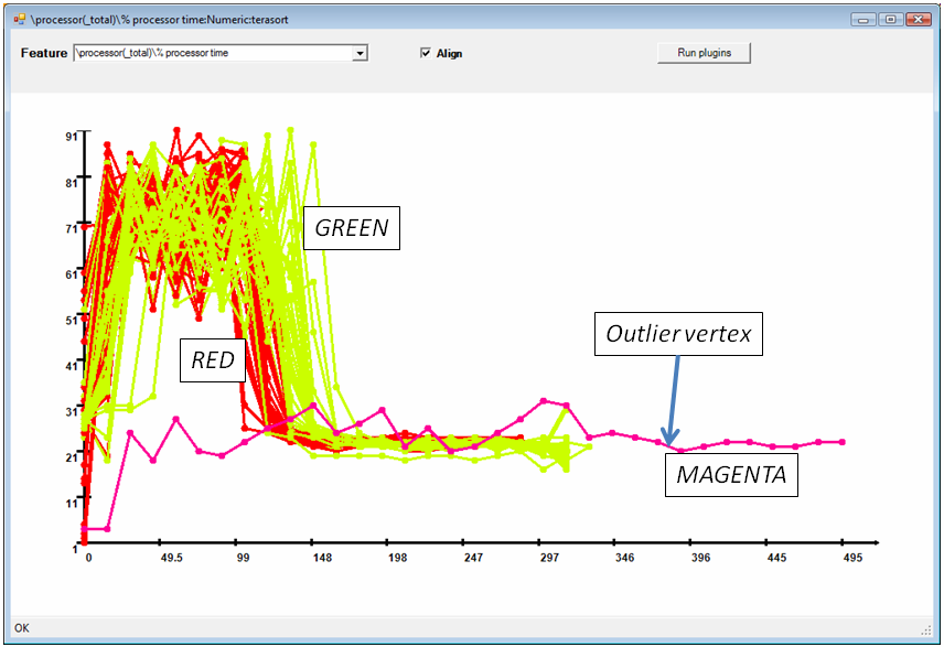
Figure 10: CPU utilization time series for selected vertices in the sorting stage.
Now we focus our attention on the magenta outlier from Figure 4, which is the long-running vertex in Figure 8. In Figure 10 we display the CPU time; we notice immediately that the outlier has much lower average CPU utilization. Integrating the CPU utilization (using the integration plug-in) we discover that the total amount of CPU used (work) is about the same for the outlier (not shown).
We then attempt to diagnose the problem by looking at the I/O rate time series, shown in Figure 11. The magenta vertex immediately stands out, since it has a much lower I/O read rate than any other vertex in the stage. Figure 6 shows that its disk I/O rate is not abnormal. But focusing on the network I/O (not shown here) we discover that the vertex is indeed reading much slower over the network compared to all its neighbors. After identifying the machine which ran this vertex we confirmed with the cluster administrator (after running some tests) that the network card on this machine was broken (the same machine is not a problem in the other stages of the sorting job, since they are not network-intensive).
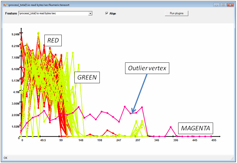
Figure 11: I/O Read bytes/second time series.
Having diagnosed the outlier, we try to understand what influences the running time in the sorting stage and what explains the difference between the “normal” sorting vertices (red and green vertices in Figure 4). We invoke the HiLighter plug-in, which runs the logistic regression to find a subset of features that predict the running time distribution (i.e., which vertices are “red” and which ones are “green”). HiLighter determines that four features related to memory management and garbage-collection predict with 92% accuracy the vertex placement in a buckets. (We confirmed this diagnosis by performing least square fitting (linear regression) with L1 to predict computation time). These four features together with one of the synthesized features -- time to reach peak CPU utilization -- predict within 5% the response time of the computation of every vertex, except for 3 outliers (out of 240 vertices). In summary, the statistical analysis indicates a strong correlation between the running time in the sorting stage and various metrics related to data size (number of garbage collection cycles, number of page faults, input size). We did not expect the input size to these vertices to have a large variance, since the data is partitioned automatically in the second job stage by the distributed sorting algorithm exactly with the purpose of load-balancing the work. By plotting the histogram of input size distribution we note that there’s a spread of 10% between the lowest and the highest input size. Since sorting is an n×log(n) algorithm, this input size difference causes a significant difference in running time. This suggests that the sampling rate of the vertices in the first computation stage in Figure 9 is too low to produce a balanced partitioning.
Artemis is appropriate (a) for executing long term studies of statistical properties of a large system, such as the ones in [7,11] and also (b) as a tool for diagnosing the performance of single run of an algorithm on a large cluster of computers. Our example in this paper illustrated its benefits in the second context.
In designing and deploying Artemis we have focused on building an extensible tool which addresses the end-to-end process of distributed log analysis, including: (a) collecting, persisting, and cleaning the raw logs; (b) computing, correlating, preprocessing and extracting features; and (c) visualizing and analyzing the data. We have relied on techniques from distributed computing, databases, visualization and statistical analysis, and machine learning.
The end-goal of this research is to provide to the end-user automatic application-specific diagnosis of performance problems. At this point Artemis handles raw data management, feature extraction and data summarization, and statistical analyses. We are currently focusing our efforts towards designing and building diagnosis plug-ins layered on the existing foundation.
Bibliography
[1] Peter Bodik, Moises Goldszmidt, and Armando Fox. HiLighter: Automatically building robust signatures of performance behavior for small- and large-scale systems. In Workshop on Tackling Computer Problems with Machine Learning Techniques (SysML), San Diego, CA, 2008.
[2] J. Bresnahan, A. Brown, D. Gunter, J. M. Schopf, M. Swany, and B. L. Tierney. Log summarization and anomaly detection for troubleshooting distributed systems. In IEEE/ACM International Conference on Grid Computing (Grid), Austin, TX, 2007.
[3] Michael Isard, Mihai Budiu, Yuan Yu, Andrew Birrell, and Dennis Fetterly. Dryad: Distributed data-parallel programs from sequential building blocks. In European Conference on Computer Systems (EuroSys), pages 59-72, Lisbon, Portugal, March 21-23 2007.
[4] Kwangmoo Koh, Seung jean Kim, Stephen Boyd, and Yi Lin. An interior-point method for large-scale L1-regularized logistic regression. Journal of Machine Learning Research, 2007.
[5] Chinghway Lim, Navjot Singh, and Shalini Yajnik. A log mining approach to failure analysis of enterprise telephony systems. In Dependable Systems and Networks (DSN), pages 398-403, Lisbon, Portugal, June 24-27 2008.
[6] Xinghao Pan, Jiaqi Tan, Soila Kavulya, Rajeev Gandhi, and Priya Narasimhan. Ganesha: Black-box fault diagnosis for MapReduce systems. Technical Report CMU-PDL-08-112, Carnegie Mellon University, September 2008.
[7] Eduardo Pinheiro, Wolf-Dietrich Weber, and Luiz Andre Barroso. Failure trends in a large disk drive population. In USENIX Conference on File and Storage Technologies (FAST), San Jose, CA, February 13-16 2007.
[8] James E. Prewett. Analyzing cluster log files using Logsurfer. In Annual Conference on Linux Clusters, 2003.
[9] James E. Prewett. Listening to your cluster with LoGS. In International Linux Cluster Conference (LCC), Austin, TX, May 2004.
[10] Daniel A. Reed, Ruth A. Aydt, Roger J. Noe, Phillip C. Roth, Keith A. Shields, Bradley W. Schwartz, and Luis F. Tavera. Scalable performance analysis: The Pablo performance analysis environment. In Scalable Parallel Libraries Conference, pages 104-113. IEEE Computer Society, 1993.
[11] Bianca Schroeder and Garth A. Gibson. A large-scale study of failures in high-performance computing systems. In Conference on Dependable Systems and Networks (DSN), pages 249-258, 2006.
[12] Jon Stearley and Adam J. Oliner. Bad words: Finding faults in Spirit's syslogs. In IEEE International Symposium on Cluster Computing and the Grid (CCGRID), pages 765-770, Washington, DC, USA, 2008.
[13] Chris Stolte, Diane Tang, and Pat Hanrahan. Polaris: A system for query, analysis, and visualization of multidimensional relational databases. IEEE Transactions on Visualization and Computer Graphics, 8(1):52-65, 2002.
[14] Wei Xu, Ling Huang, Armando Fox, David Patterson, and Michael Jordan. Mining console logs for large-scale system problem detection. In Workshop on Tackling Computer Problems with Machine Learning Techniques (SysML), San Diego, CA, 2008.
[15] Yuan Yu, Michael Isard, Dennis Fetterly, Mihai Budiu, Ulfar Erlingsson, Pradeep Kumar Gunda, and Jon Currey. DryadLINQ: A system for general-purpose distributed data-parallel computing using a high-level language. In Symposium on Operating System Design and Implementation (OSDI), San Diego, CA, December 8-10 2008.
[1]“Application-specific” parts depend on the specific distributed application that we are trying to analyze.
[2] From Wikipedia: Dryads are tree nymphs in Greek mythology. They are normally considered to be very shy creatures, except around the goddess Artemis, who was known to be a friend to most nymphs. Artemis is also the Hellenic goddess of the hunt.
[3] If some of the cluster machines are unavailable, the data collection will still succeed, but produce incomplete data.
[4] In this context “cluster” refers to a data cluster – a grouping of data according to a clustering algorithm.
[5] In order to process just the sorting stage we first use a histogram of stages (one bucket per stage – projecting the view on stage), and then we select just the sorting stage (selecting the suitable checkbox).