Songyun Duan and Shivnath Babu
Department of Computer Science, Duke University
Automated techniques to diagnose the cause of system failures based on monitoring data is an active area of research at the intersection of systems and machine learning. In this paper, we identify three tasks that form key building blocks in automated diagnosis:
We provide (to our knowledge) the first apples-to-apples comparison of both classical and state-of-the-art techniques for these three tasks. Such studies are vital to the consolidation and growth of the field. Our study is based on a variety of failures injected in a multitier Web service. We present empirical insights and research opportunities.
Failures of Internet services and enterprise systems lead to user dissatisfaction and considerable loss of revenue. Manual diagnosis of these failures can be laborious, slow, and expensive. This problem has received considerable attention recently from researchers in systems, databases, machine learning and knowledge discovery, computer architecture, and other areas (e.g., [2,5,6,7]). The research has been directed at developing automated, efficient, and accurate techniques for diagnosing failures using system monitoring data. These techniques are based on one or both of two fundamental primitives in machine learning: (i) clustering, which partitions data instances into groups based on similarity; and (ii) classification, which predicts the category of data instances based on attribute values.
While clustering and classification are well-studied problems, applying them in the context of automated diagnosis poses nontrivial challenges like:
This paper compares some classical as well as some more recent techniques that have been developed to address such challenges. For this comparison, we identify three tasks that form key building blocks in automated diagnosis. The tasks are presented in Section 2 along with the details of system monitoring data. The techniques we evaluate for each task are presented in Section 3. Our evaluation is based on an implementation of all techniques in the Fa system-management platform being developed at Duke [9,10,11].1
The evaluation setting is a testbed that runs the Rubis [13] auction Web service where we inject failures caused by factors like software bugs, data corruption, and uncaught Java exceptions. Section 4 presents the evaluation setting, methodology, and results. We conclude in Section 5.
System Monitoring Data:
When a system is
running, Fa collects monitoring data periodically and stores it
in a database. In this paper, we consider monitoring data having a
relational (row and column) schema with
attributes ![]() ,
, ![]() ,
, ![]() . For example, Fa
collects more than a hundred
performance metrics (e.g., average CPU utilization, number of
disk I/Os) periodically from Linux servers.
Application servers and database servers
maintain performance counters (e.g., number of invocations
of each Java module, number of index updates,
number of full table scans) that Fa reads periodically. Most
enterprise monitoring systems like HP OpenView and IBM Tivoli
Monitoring collect similar data.
. For example, Fa
collects more than a hundred
performance metrics (e.g., average CPU utilization, number of
disk I/Os) periodically from Linux servers.
Application servers and database servers
maintain performance counters (e.g., number of invocations
of each Java module, number of index updates,
number of full table scans) that Fa reads periodically. Most
enterprise monitoring systems like HP OpenView and IBM Tivoli
Monitoring collect similar data.
Over a period of time, the historic monitoring data collected by Fa will contain two types of instances:
Apart from
![]() , the monitoring data contains
an annotation attribute
, the monitoring data contains
an annotation attribute ![]() . The value of
. The value of ![]() in an instance
indicates whether the instance belongs to
in an instance
indicates whether the instance belongs to ![]() or
or ![]() .
We consider three tasks that process the system monitoring
data in different ways to aid failure diagnosis.
.
We consider three tasks that process the system monitoring
data in different ways to aid failure diagnosis.
Task I: Identifying distinct system states. This capability helps system administrators in many ways. For example, administrators can understand the evolving behavior of the system, or identify baseline system behavior from the different healthy states of a dynamic system. Furthermore, administrators can prioritize their diagnosis efforts by identifying the frequent failure states and the associated revenue losses.
Task II: Retrieving historic instances from the monitoring data that are similar to one or more given instances. This capability helps system administrators leverage past diagnosis efforts for recurrent failures. Failure diagnosis is expensive in complex systems, so it is valuable to leverage past diagnosis efforts whenever possible; particularly since 50-90% of failures seen are recurrences of previous failures [3]. Furthermore, identifying similar instances from the past helps generate more data that can be input to machine-learning tools. These tools usually give more accurate and confident results when more input (training) data is provided.
Task III:
Processing a diagnosis query
Diagnose![]() . Here,
. Here, ![]() consists of monitoring instances
from a healthy system state, while
consists of monitoring instances
from a healthy system state, while ![]() consists
of instances from a failure state. The result of this
query is a selected subset of attributes in the monitoring data
that indicate the likely cause of the failure represented
by
consists
of instances from a failure state. The result of this
query is a selected subset of attributes in the monitoring data
that indicate the likely cause of the failure represented
by ![]() . While Task III is the quintessential task of automated diagnosis, it
may need the results of Tasks I and II to generate the inputs
. While Task III is the quintessential task of automated diagnosis, it
may need the results of Tasks I and II to generate the inputs
![]() and
and ![]() .
.
We briefly describe the techniques that were implemented and compared for the three tasks above. Please refer to the cited original papers for the full details of each technique.
The main approach used for solving this task is to divide the
historic monitoring data ![]() into non-overlapping partitions
such that instances in each partition have similar
characteristics that represent a distinct system state. The
frequency of a state can then be estimated as the
size of the corresponding partition.
into non-overlapping partitions
such that instances in each partition have similar
characteristics that represent a distinct system state. The
frequency of a state can then be estimated as the
size of the corresponding partition.
We can partition data using a classical clustering technique like K-Means. However, recent work observes that clustering techniques like K-Means suffer from the curse of dimensionality in high dimensional spaces [8]. In such spaces, for any pair of instances within the same cluster, it is highly likely that there are some attributes on which the instances are distant from each other. Thus, distance functions that use all input attributes equally can be ineffective. Furthermore, different clusters may exist in different subspaces, i.e., comprised of different subsets of attributes [8].
These issues are addressed by
subspace clustering (e.g., [1,8]) which
discovers clusters in subspaces defined by
different combinations of attributes.
The locally adaptive clustering (LAC) algorithm from [8]
associates each cluster ![]() with a
weight vector that reflects the correlation among
instances in
with a
weight vector that reflects the correlation among
instances in ![]() . Attributes on which the instances in
. Attributes on which the instances in ![]() are strongly
(weakly) correlated receive a large (small) weight,
which has the effect of constricting (elongating) distances along
those dimensions.
are strongly
(weakly) correlated receive a large (small) weight,
which has the effect of constricting (elongating) distances along
those dimensions.
Extension of the Clustering
Process
Reference [7] uses K-Means (with ![]() =
=![]() ) as
a building block to produce pure clusters iteratively.
The purity of a cluster is defined based on the annotation attribute:
a cluster is completely pure if it
contains failure instances only or it contains healthy
instances only. (We will later extend
the definition of purity to multiple different
failure types.) The extended clustering process in [7]
works as follows:
) as
a building block to produce pure clusters iteratively.
The purity of a cluster is defined based on the annotation attribute:
a cluster is completely pure if it
contains failure instances only or it contains healthy
instances only. (We will later extend
the definition of purity to multiple different
failure types.) The extended clustering process in [7]
works as follows:
The authors of [7] explore the space of
possible values for ![]() to compare the clustering
techniques.
to compare the clustering
techniques.
A classification tree (CART, or decision tree) [14]
can be learned from the historic data ![]() with
the annotation attribute as the class attribute, and the others as
predictor attributes. The tree's leaf nodes represent
a partitioning of the data. A nice feature of this
approach--which arises from its roots in classification as opposed
to clustering--is that the tree minimizes the chances of putting instances from
healthy states and instances from failure states into the same
partition. We can vary the pruning level [14]
of the tree during learning
to generate different numbers of partitions (leaf nodes) from
with
the annotation attribute as the class attribute, and the others as
predictor attributes. The tree's leaf nodes represent
a partitioning of the data. A nice feature of this
approach--which arises from its roots in classification as opposed
to clustering--is that the tree minimizes the chances of putting instances from
healthy states and instances from failure states into the same
partition. We can vary the pruning level [14]
of the tree during learning
to generate different numbers of partitions (leaf nodes) from ![]() .
(Pruning is usually used to avoid overfitting the training data.)
More aggressive pruning will generate a tree with fewer
leaf nodes (partitions).
.
(Pruning is usually used to avoid overfitting the training data.)
More aggressive pruning will generate a tree with fewer
leaf nodes (partitions).
Given an instance ![]() , we can retrieve the top
, we can retrieve the top
![]() historic instances from
historic instances from
![]() that are the most similar to
that are the most similar to ![]() . The similarity between two
instances
. The similarity between two
instances ![]() and
and ![]() can be measured by the inverse of their
pairwise Euclidean distance.
can be measured by the inverse of their
pairwise Euclidean distance.
The retrieval of ![]() based on a CART learned from historic data
will return all instances from the leaf node that the CART
classifies
based on a CART learned from historic data
will return all instances from the leaf node that the CART
classifies ![]() into. The intuition here
is that the returned instances have similar patterns in attribute
values (i.e., satisfy a similar set of conditions) as
into. The intuition here
is that the returned instances have similar patterns in attribute
values (i.e., satisfy a similar set of conditions) as ![]() .
.
Given a diagnosis query
![]() ,
where
,
where ![]()
![]()
![]() and
and ![]() contains
instances during or just before a failure, the task of
processing this query is to track down the subset of attributes that
pinpoint the cause of the failure represented by
contains
instances during or just before a failure, the task of
processing this query is to track down the subset of attributes that
pinpoint the cause of the failure represented by ![]() .
Previous techniques for processing Diagnose
.
Previous techniques for processing Diagnose![]() belong to
one of the following two categories:
belong to
one of the following two categories:
We now describe the techniques compared for Task III.
The metric-attribution approach from Reference [6]
processes a
![]() query as follows:
query as follows:
The CART-based diagnosis approach [5] works as follows:
The baselining-based approach described in [2]
first captures the distribution ![]() of attribute
of attribute ![]() 's (
's (
![]() ) values in the healthy instances
) values in the healthy instances ![]() .
. ![]() is approximated by a Gaussian distribution in
[2]. Then, [2] computes the
probability of
is approximated by a Gaussian distribution in
[2]. Then, [2] computes the
probability of ![]() having produced the measurements of
having produced the measurements of ![]() in the failure instances
in
in the failure instances
in ![]() . If this probability is lower than a threshold, then
. If this probability is lower than a threshold, then ![]() is
included in the diagnosis result.
is
included in the diagnosis result.
The techniques discussed so far for the three tasks work directly on the raw monitoring data. Reference [7] applies metric attribution (Section 3.3.1) to construct a signature for each instance in the historic data. (This approach is one example of applying transformations to the raw data.) The signature of an instance aims to distill the system state that the instance belongs to. Partitioning and retrieval can be done with the constructed signatures instead of the raw data, with the hope that the quality of results for Tasks I and II will be improved. Signatures are constructed as follows:
We evaluate the techniques described in this paper in the context of common failures in a three-tier Web service. We implemented a testbed that runs Rubis [13]--a multitier auction service modeled after eBay--on a JBoss application server (with an embedded Web server) and a MySQL DBMS. It has been reported that software problems and operator errors are the common causes of failure in Web services [12]. We inject such failures into a running Rubis instance using a comprehensive failure-injection tool [4]. This setting makes it easy to study the accuracy of various diagnosis algorithms because we always know the true cause of each failure.
Specifically, we can inject 3 independent causes of failure--software bugs, data corruption, and uncaught Java exceptions--into 25 Java modules (Enterprise Java Beans (EJBs)) that comprise the part of Rubis running in the application server. Using this mechanism, we can inject 75 distinct single-EJB failures and any number of independent multiple-EJB failures (concurrent single-EJB failures).
We collect data for each failure type ft as follows: (1) run the testbed under a stable workload (there is no performance bottleneck for this workload) for 20 minutes; (2) inject the specific failure ft into the testbed and continue the run for 20 minutes; (3) fix the failure by microrebooting [4] affected EJBs, and go to Step 2. The whole process lasts 200 minutes. The monitoring data used in the evaluation consists of the number of times each distinct EJB procedure call is invoked per minute; consisting of a total of 110 attributes. (Monitoring at this level is light-weight.) SLO violations are defined based on Rubis's average response time per-minute. For evaluation purposes, we assign an annotation to each data instance being collected as follows: (i) healthy, if the instance has no SLO violation, or (ii) the identifier of the injected failure type, if the instance has SLO violations. A failure type is defined by which causes of failure were injected into which EJBs.
The Rubis-5, Rubis-10, and Rubis-20 monitoring datasets in Table 1 are used in the evaluation. All experiments were run on a machine with 2 GHz CPU and 1 GB memory.
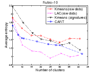
The entropy formula from Section 3.1.1
can be generalized to multiple annotations as
![]() , where
, where ![]() is the percentage of
instances with a specific annotation in a cluster. The quality
of a partitioning result can be measured as the average entropy
over all produced clusters weighted by their normalized cluster
sizes. Generally, the lower the average entropy, the better the partitioning.
An average entropy close to 0 means that each cluster mostly
contains instances from one system state; so the partitioning
characterizes different system states correctly.
is the percentage of
instances with a specific annotation in a cluster. The quality
of a partitioning result can be measured as the average entropy
over all produced clusters weighted by their normalized cluster
sizes. Generally, the lower the average entropy, the better the partitioning.
An average entropy close to 0 means that each cluster mostly
contains instances from one system state; so the partitioning
characterizes different system states correctly.
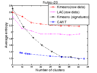
We compare four partitioning techniques: (1) K-means applied on the raw monitoring data, (2) LAC applied on the raw monitoring data, (3) K-means applied on signatures constructed from the monitoring data, and (4) CART. Recall from Section 3.4 that we need to set the chunk size for signature construction. We set the chunk size to 100 to ensure that each chunk has sufficient healthy and failure instances to learn a reasonable Bayesian network. We do not have a direct control over the number of partitions generated by CART. We can only vary the pruning level that affects how many leaf nodes (partitions) remain in the produced tree.
Figures 1 and 2 show the average entropy of each partitioning technique as we increase the number of maximum allowed partitions for Rubis-10 and Rubis-20 respectively. We observe the following trends:
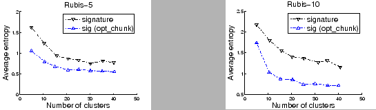
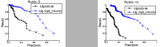
To verify our observations about signatures, we analyzed the possible improvement when the chunk size is set optimally (which is possible only when we know the points where system resources, workload, or configuration changed). Figure 3 plots the average entropy of K-means clustering on signatures for Rubis-5 and Rubis-10 respectively in two settings: (1) the chunk size is fixed at 100 during signature construction (denoted as signature); and (2) the chunk size is set adaptively to capture all change points in system state (denoted as sig(opt_chunk)). Note the considerable improvement in the quality of partitioning with optimal chunk sizes. The relative improvement also increases as the number of failure types increase.
We adopt the traditional metrics of precision and recall for
evaluating retrieval quality. For a given instance
![]() and number
and number ![]() of instances similar to
of instances similar to ![]() to be retrieved:
precision measures the percentage of correctly-retrieved
instances among the
to be retrieved:
precision measures the percentage of correctly-retrieved
instances among the ![]() results;
and recall measures the percentage of correctly-retrieved instances
among all historic instances with the same annotation as
results;
and recall measures the percentage of correctly-retrieved instances
among all historic instances with the same annotation as ![]() .
The perfect value for both metrics is 100%.
Intuitively, as
.
The perfect value for both metrics is 100%.
Intuitively, as ![]() increases,
recall improves while precision drops. Thus,
the bigger the area under the precision-recall
curve, the better.
increases,
recall improves while precision drops. Thus,
the bigger the area under the precision-recall
curve, the better.
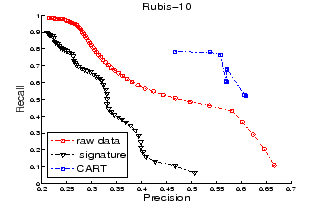
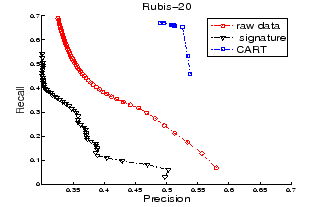
Figures 4 and 5 plot the
precision-recall curves for Rubis-10 and Rubis-20 respectively.
![]() is varied from 20 to 1000.
The precision and recall values are averaged
over a test set comprising 40% of the data.
We could not plot the precision-recall curve for CART in
the high-recall and high-precision regions since
we do not have direct control on the number of instances
retrieved from a CART (recall Section 3.2).
is varied from 20 to 1000.
The precision and recall values are averaged
over a test set comprising 40% of the data.
We could not plot the precision-recall curve for CART in
the high-recall and high-precision regions since
we do not have direct control on the number of instances
retrieved from a CART (recall Section 3.2).
Reference [7] observed that signature-based retrieval is better than raw-data-based retrieval. However, Figures 4 and 5 show contrary results. Once again, the possible reason is that signature construction is sensitive to the chunk-size setting; but there is no principled way to set this value statically. This point is verified in Figure 6 which shows the precision-recall curves for Rubis-5 and Rubis-10 for the fixed chunk-size and optimal chunk-size settings (recall Section 4.1). There is considerable improvement in both precision and recall with optimal chunk sizes.
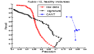
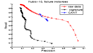
Retrieval based on CART performs better than the other two techniques because CART retrieves healthy instances with higher precision than the other two. This point is verified in Figures 7 and 8 which respectively plot the precision-recall curves for retrieving healthy instances only and failure instances only in Rubis-10.
Since we know the actual root cause of each failure injected in the testbed, we can evaluate the accuracy of a diagnosis technique in terms of the false positives (FP) and false negatives (FN) in its result. FP counts the number of EJBs that appear in the diagnosis result but are not the root cause of failure. FN counts the number of EJBs that cause the failure but are missing from the diagnosis result. Both false positives and false negatives hurt diagnosis accuracy.
Table 2 compares the diagnosis accuracy of the three techniques: metric attribution (MA), CART, and anomaly detection (AD). The failures were injected one at a time, and come from a combination of ten distinct EJBs and three distinct failure types: Java exceptions (Exception), data corruptions (jndi), and software bugs (nullmap). (Table 2 shows a subset of the results.) MA performs slightly better than the other two techniques in capturing the root cause. MA fails 10 out of 30 times to catch the true cause (FN = 1). However, MA tends to produce more false positives than CART. A good combination of these techniques may reduce both false positives and false negatives. A manual analysis of the results showed that FP can be reduced by incorporating domain knowledge--e.g., inter-EJB calling patterns which lead to fault propagation [4]--alongside the statistical machine-learning analysis.
|
We empirically compared techniques for three tasks related to diagnosis of system failures. While a number of empirical insights were generated, there was no dominant winner among the techniques we compared. Our evaluation showed plenty of room for improving these techniques in the following aspects to realize industrial-strength automation of failure diagnosis, and to ultimately make systems detect, diagnose, and fix failures automatically ( self-healing):
We are extremely grateful to Carlotta Domeniconi for providing us the source code for LAC, and to George Candea and other members of Stanford's Software Infrastructure Research Group for helpful discussions and source code.
This document was generated using the LaTeX2HTML translator Version 2002-2-1 (1.71)
Copyright © 1993, 1994, 1995, 1996,
Nikos Drakos,
Computer Based Learning Unit, University of Leeds.
Copyright © 1997, 1998, 1999,
Ross Moore,
Mathematics Department, Macquarie University, Sydney.
The command line arguments were:
latex2html -split 0 -show_section_numbers -local_icons -no_navigation paper.tex
The translation was initiated by Songyun Duan on 2008-11-23