
|
1RAD Lab, EECS Department, UC Berkeley, | 2Microsoft Research, Silicon Valley |
Previous work showed that statistical analysis techniques could successfully be used to construct compact signatures of distinct operational problems in Internet server systems. Because signatures are amenable to well-known similarity search techniques, they can be used as a way to index past problems and identify particular operational problems as new or recurrent. In this paper we use a different statistical technique for constructing signatures (logistic regression with L1 regularization) that improves on previous work in two ways. First, our new approach works for cases where the number of features is an order of magnitude larger than the number of samples and also scales to problems with over 50,000 samples. Second, we get encouraging results regarding the stability of the models and the signatures by cross-validating the accuracy of the models from one section of the data center on another section. We validate our approach on data from an Internet service testbed and also from a production enterprise system comprising hundreds of servers in several data centers.
Interactive network services experience performance problems for a wide variety of reasons. Diagnosing these problems is complicated due to various factors including the large scale deployment of these services, their complex interactions, and the large number of metrics collected in each component of the system.
The work in [2] proposed an approach to alleviate the diagnosis problem by automatically building a compact signature of each failure mode. These signatures are then used to a) localize the problem (sometimes establishing a path to the root cause), b) detect recurring instances of the same problem, and c) serve as indexes for annotations regarding resolution. The applications b) and c) were addressed using a similarity search over the signatures, effectively reducing problem identification to information retrieval. The automatic construction of these signatures in [2] is based on classification with feature selection to find subsets of measured system metrics (CPU, memory utilization, etc.) that were correlated with the performance problem. The signature of a particular instance of a problem is then extracted by finding whether each of the selected features contributes to classifying the instance as anomalous or as normal. The paper then demonstrated the benefits of this approach on a transactional system consisting of tens of geographically-distributed servers.
In this paper we revise the methodology for inducing a classifier and selecting the features. While the work in [2] relied on a Bayesian network classifier and a heuristic search over the space of features, we use logistic regression with L1 regularization [6][7]. The first advantage of using this approach is that it works well in cases where the number of features being considered exceeds the number of samples; Case Study 1 describes an example with over 2000 features and only 86 datapoints. An example of such a scenario is application testing, where thousands of features are collected per machine, yet the number of samples in a particular failure mode is limited by the duration of the test run. The second advantage is the availability of very efficient implementations of L1-regularized regression that scale to datasets with tens of thousand samples, which is a requirement for an application in a cloud computing environment with thousands of machines. We built a tool called HiLighter based on the algorithm and C# implementation for regularized log-linear models described in [1].
To demonstrate and validate HiLighter we applied it to data from a testbed of an Internet service, where the number of features is an order of magnitude higher than the number collected samples. This testbed is used in the service product group to test and validate new features in the product. We also applied HiLighter to data from two known performance problems in a production environment with hundreds of machines, each reporting hundreds of metrics. Three interesting results emerge. First, we were able to help diagnose a problem in the testbed using HiLighter. This is notable since the approach in [2] would be unable to reliably fit a model under those conditions. Second, we get encouraging results by cross-validating the accuracy of the models from one group of servers in a datacenter on a new group of servers. Given that the signatures are extracted from the models in a deterministic fashion, the results suggest that the signatures being computed as "digests" of the problem states are stably capturing the metrics relevant to each problem. Finally, we observe stable and distinct signatures for the system's state just before and after the performance problem as well. This suggests that signatures can be used not only to identify a particular performance problem but possibly to forecast it almost an hour in advance. We are currently working with human experts on verifying the forecasting possibilities. The group responsible for the service whose data was analyzed have incorporated the code for HiLighter to their code tree for integration with their other tools.
We first present the details of the HiLighter algorithm, followed by three case studies: one from an application testbed and two from a large-scale production environment.
We start by reviewing the classification model and feature selection approach used by HiLighter and then we contrast these with the approaches in [2]. HiLighter is based on a logistic regression classifier. A logistic regression model is a common statistical parametric approach based on the assertion that the class variable Y is a Bernoulli random variable with mean pj [8], where 1 <= j <= m is the jth sample.1 Given the set of features M, the model is given by p_j = P(Y_j = 1|M_j = m) = (exp(SUM_i beta_i m_i))/(1+ exp(SUM_i beta_i m_i)) Usually, the parameters betai are fitted by maximizing the likelihood function L(beta) = PRODj pjYj(1-pj)1-Yj. The L1 regularization extends the objective function to include the constraint that the L1 norm of the parameters be less than a value lambda; that is, SUM|betai| <= lambda, where lambda can be fitted in a variety of ways including cross-validation. Because the first partial derivative of the L1 regularizer with respect to each beta coefficient is constant as the coefficient moves toward zero, the values of the coefficients are "pushed" all the way to zero if possible. For more formal justifications we refer the reader to [7][6][1]. This regularization was shown theoretically and experimentally to learn good models even when most features are irrelevant and when the number of parameters is comparable to the number of samples [7][6]. It also typically produces sparse coefficient vectors in which many of the coefficients are exactly zero and can thus be used for feature selection.
In contrast, the feature selection approach in [2] was based on a greedy search process wrapped around an induction of a Bayesian network classifier [4], which has two immediate consequences. First, because the search considers changes to one feature at a time in a greedy neighborhood, the explored search space is severly constrained and in large problems only a small subspace is explored. Second, the inner loop of the feature selection requires a model selection step such as cross-validation which introduces another source of error.2 By relying on the gradient of the likelihood function, the logistic regression with L1 regularization performs a guided exploration of a much larger part of the search space.
We adapt the methodology in [2] to our setting to construct signatures of performance problems. In each time quantum, the system collects hundreds of performance metrics reported by the hardware, operating system (Windows Server), runtime system (Microsoft Common Language Runtime), and the application itself. The operators of the service specify one of these performance metrics as a "metric of merit" (e.g., average response time) and we define a class for each time interval as normal or abnormal, depending on whether the metric of merit exceeds some chosen threshold during that interval.
The first step in constructing the signatures for a performance anomaly is a selection of a small number of metrics that well predict both normal and abnormal performance with high accuracy. HiLighter transforms the measured metrics using standard preprocessing: a) removes the constant metrics, b) augments each metric by computing a gradient and standard deviation with respect to one or two time periods in the past (thereby creating additional features), and c) normalizes the metrics to zero mean and variance of one. For now, we simply remove entries for which data is missing; this was not a factor in Case Study 1, but it affected Case Study 2, as described in Section *.
As recommended in [2], we evaluate the models using Balanced Accuracy, which averages the probability of correctly classifying normal with probability of detecting an anomaly; this is necessary since there are typically many more instances of normal performance than anomalous performance. The number of metrics selected is affected by a lambda parameter which is the contraint on the L1 regularization. There are many ways to find lambda that achieves the optimal classification accuracy [9]; HiLighter uses five-fold cross-validation in conjunction with a binary search over the values of lambda.
After the feature selection using L1, HiLighter fits the final model using the selected metrics and adds an L2 constraint to stabilize for correlated features (as recommended in [9]). HiLighter then reports balanced accuracy, the confusion matrix including false positives and false negatives, and the balanced accuracy of using each metric alone as a classifier. As will be apparent in Case Study 2 and 3, the balanced accuracy of the final model with multiple metrics is significantly better than the balanced accuracy of a model with just one or two metrics, clearly making the case for models that take into account the interaction among features.
Finally, we use the selected metrics to construct a signature of each machine at each time interval. A signature consists of the list of the selected metrics, where we label each metric as abnormal if its value contributes positively to the classification of this machine as abnormal; otherwise we label the metric normal. Formally, metric i is labeled abnormal if mi * betai > 0, where mi is the value of metric i and betai is the coefficient in the linear classifier corresponding to this metric. Such a signature serves as a condensed representation of the state of the machine at the given time interval.
The first case study concerns a multi-tier Internet application deployed across multiple datacenters. We examined traces from a small-scale testbed used for testing new features and capabilities of the application. The traces contained the following types of metrics measured every 30 seconds: workload, response times, OS-level metrics, .NET runtime metrics, and application-specific metrics. After the feature extraction process in HiLighter, the dataset contained about 1000 features per server.
The performance anomaly we investigated was large variance in the 99th percentile of latency under steady workload and stable external environment. The values of latency were ranging from 50 to 1200 ms, in clear contrast to an identical run on a separate set of servers where the response time stayed below 300 ms. We found that a threshold of 400 ms clearly separated the slow, anomalous requests from the normal ones. We included metrics from one first-tier and one second-tier server, since each request passed through both types of server. The resulting dataset contained only 86 datapoints and 2008 features, from which HiLighter selected just two metrics, both reported by the .NET runtime: number of induced garbage collections and change in number of allocated bytes. The resulting model reached cross-validated balanced accuracy of 0.94 which strongly suggests that garbage collection was the cause of this performance anomaly. We note that we tried all major classifiers, including Naive Bayes and Support Vector Machines, with feature selection as implemented in Weka [5] with little success.
The second case study focuses on a performance issue in the production version of another large-scale Internet application. This application is deployed across six datacenters with hundreds of servers, each serving one of five roles in the overall application. The "application core" servers--call them Role 1 servers--contain the main application logic, and each of these servers measures the average latency of requests it processed. The performance problem we investigated was triggered by a deployment of a bad configuration file to all Role 1 servers, resulting in significant processing delays of the received requests.
We used HiLighter on data from four groups of Role 1 servers housed in datacenter 5; each group contained between 20 and 70 servers. The feature extraction process resulted in a dataset with approximately 500 metrics and 100 datapoints per server and time interval. We used the average latency on each server as our reference metric and used a threshold supplied by operators of this service. The linear models produced by HiLighter selected between six and nine metrics and achieved cross-validated balanced accuracy between 0.92 and 0.95. The selected metrics were a combination of CPU utilization, internal workloads, and other application-specific measures. When comparing models that used exactly six metrics, five of the metrics selected by the different models were identical, thus, the models would generate almost identical signatures. The number of metrics selected can heavily influence model accuracy: in one group of servers, the balanced accuracy increased from 0.83 with only two metrics to 0.92 with six metrics, further confirming the need to consider interactions among metrics rather than just the contributions of individual metrics.
Despite using data from the same anomaly, there were notable differences in the metrics selected for each model. These differences could mean that the models wouldn't generalize to other instances of this anomaly, which would decrease their usefulness. To test the accuracy of the models on new instances of this anomaly, we separately evaluated each of the models on data from the remaining three groups of servers. As summarized in Table *, the balanced accuracy was between 0.90 and 0.96 which demonstrates that the models could accurately detect this anomaly. We believe that the differences in selected metrics are due to missing values in our dataset; we omitted metrics with too many values missing and these thus couldn't be selected by HiLighter. Later the operators of the service informed us that the missing data points actually represent a values of zero. After replacing the missing values with zeros, the metrics selected in different groups of servers were almost identical.
Knowing which other server roles were affected by this anomaly could considerably help the operators during root cause analysis. We therefore used HiLighter on the other four types servers (roles two through five) grouped by datacenter and role. However, because these servers don't measure latency as the role 1 servers do, we used timestamps to define the anomaly. That is, the anomaly is defined to have occurred during the time period in which the role 1 servers were reporting poor request latency.
As summarized by Table *, for some groups of servers, such as role 5 in datacenter 6, the balanced accuracy was very low, suggesting that (metrics reported by) these servers were not affected by this issue. However, most of the other server groups seem to have been affected and analyzing the selected metrics would likely aid the operators in diagnosing this issue.
We constructed signatures as defined in Section * for a group of 71 servers and analyzed how these signatures evolved before, during, and after the anomaly (see Figure *). HiLighter selected six metrics for the model: three measures of CPU utilization (features 1-3), number of connections and disconnections on an internal component in the server (features 4-5), and the variance of workload on another internal component (feature 6). As described in Section *, given a model of the anomaly, a signature is constructed for every data point, i.e. for each server and time interval. The signature consists of the metrics selected for the model and a binary label for each metric. A + label means that the value of the metric is abnormal relative to the model, a - label means the metric is normal.
The changes in signatures over time help us understand what happened during the anomaly. To simplify the visualization of signatures in Figure *, we clustered the signatures into four groups based on the number of abnormal metrics. Signature group A (dark gray) contains signatures with at most two abnormal metrics; signature B (light gray) has all metrics abnormal except metric 6; signature C (black) has all metrics abnormal; and group other represents all remaining signatures. The figure clearly shows that signatures in group A were prevalent up to about 14 intervals before the start of the anomaly and then again 14 intervals after the end of the anomaly. Despite containing some anomalous metrics, the HiLighter model correctly predicted normal. Signature C corresponds to the anomaly itself, and since all the metrics are anomalous, the model correctly predicted anomaly. However, up to 14 intervals before and after the anomaly, signature B was most prevalent, which suggests that five out of the six chosen metrics were already "misbehaving" long before the measured anomaly started. The anomaly of individual metrics caused a significant number of false positives in the results of the HiLighter model. We hypothesize that further characterizing signature B would allow us to predict such anomalies in the future.
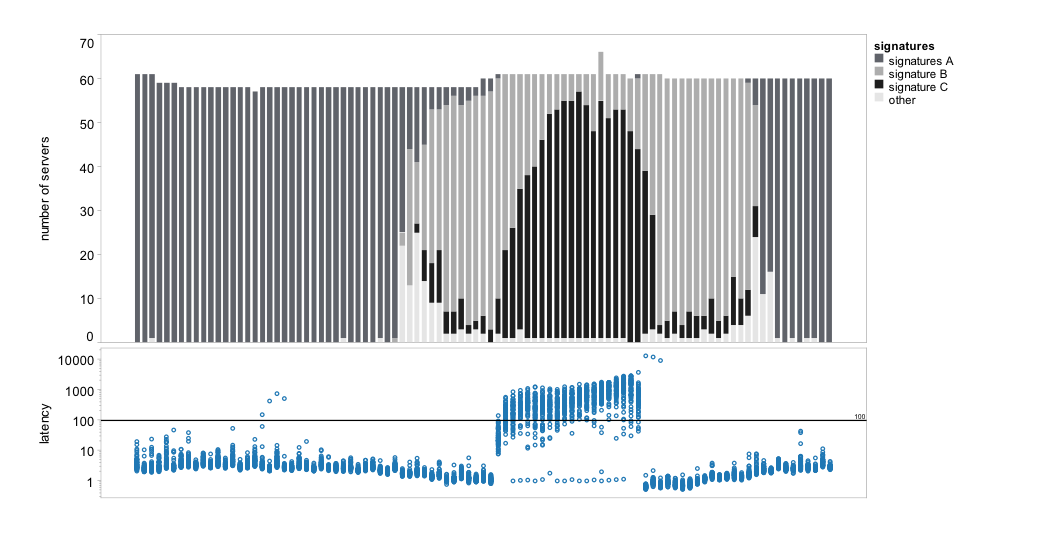 The bottom plot shows the latency as measured by the 71 role-one servers over time; each dot represents latency on one server during a single time interval. The anomaly is visible in the middle part of the plot. The top plot shows the evolution of signatures over time on all the servers; on average, for ten out of the 71 servers we cannot compute signatures because of missing values.
| gr. 1 | gr. 2 | gr. 3 | gr. 4 | |
| group 1 | 0.92 | 0.93 | 0.92 | 0.91 |
| group 2 | 0.95 | 0.95 | 0.96 | 0.94 |
| group 3 | 0.92 | 0.92 | 0.95 | 0.92 |
| group 4 | 0.90 | 0.90 | 0.92 | 0.93 |
| DC 1 | DC 2 | DC 3 | DC 4 | DC 5 | DC 6 | |
| role 1 | 0.92 | 0.95 | 0.99 | 0.92 | ||
| role 2 | 0.96 | 0.99 | 0.85 | 0.67 | 0.97 | |
| role 3 | 0.93 | |||||
| role 4 | 0.80 | |||||
| role 5 | 1.00 | 0.52 | ||||
| gr. 1 | gr. 2 | gr. 3 | gr. 4 | |
| group 1 | 0.97 | 0.97 | 0.96 | 0.96 |
| group 2 | 0.98 | 0.99 | 0.98 | 0.98 |
| group 3 | 0.96 | 0.95 | 0.99 | 0.99 |
| group 4 | 0.95 | 0.92 | 0.96 | 0.96 |
In the last case study we analyze another performance issue in the same application. One of its datacenters was overloaded, which caused significant processing delays as external traffic was redirected to the remaining datacenters. After feature extraction we obtained a dataset of approximately 500 features and 100 datapoints per server. We used HiLighter on the same four groups of Role 1 servers as in Case Study 2, and evaluated each model on data from the remaining three groups. As summarized in Table *, with one exception, accuracy of the models was in the range of 0.95 and 0.99. Three out of the four metrics selected by the different models were identical and thus the models would generate almost identical signatures.
As in Case Study 2, we analyzed the evolution of the signatures for the group of 71 Role 1 servers. The HiLighter model selected for this group of servers includes CPU utilization (feature 1) and variance of four internal workload metrics (features 2-5). Figure * shows the behavior over time (normal vs. abnormal with respect to the performance model) of the five individual features. This visualization allows us to easily spot when each metric became abnormal and how many servers were affected. Metrics 2, 3 and 5 capture the duration of the anomaly very well, but the anomaly in CPU utilization (metric 1) precedes the start of the performance issue. We hypothesize that this signature could be used in the future to predict the occurrence of such anomalies. One troublesome issue is the behavior of metric 4, which becomes abnormal long before the anomaly starts. However, since it is the only anomalous metric, HiLighter's model correctly predicts normal overall state of the system, and reports only a single false negative at the beginning of the dataset.
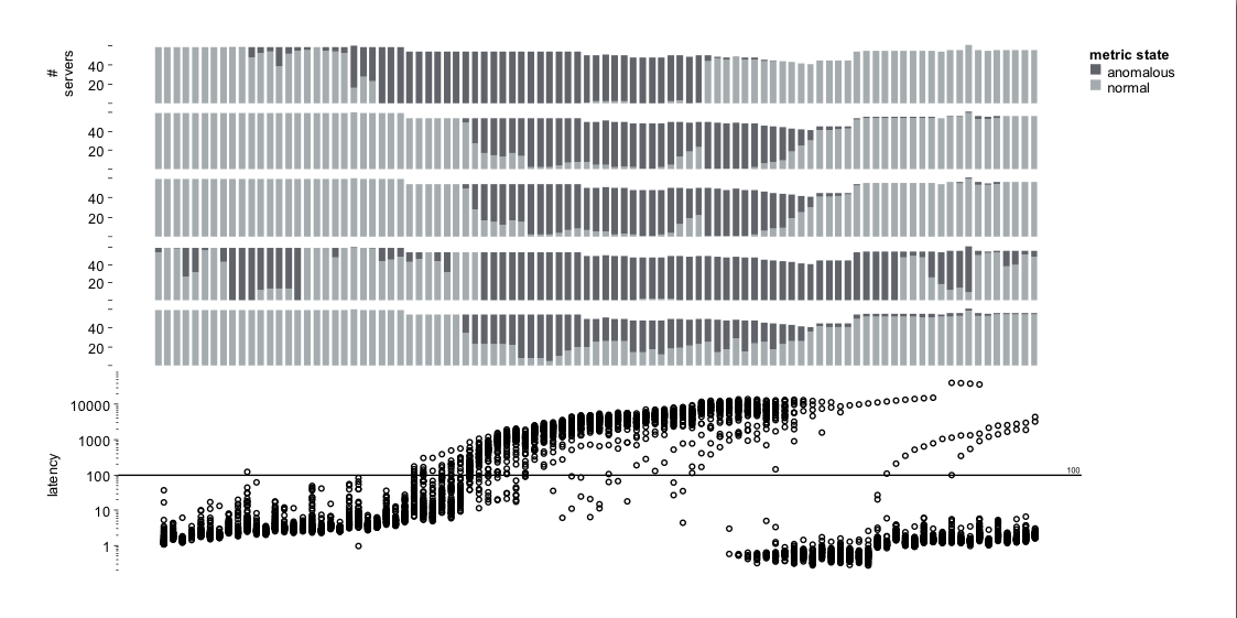 As in Figure *, the bottom plot shows the latency on the 71 role-one servers. The plots on the top show the state of each of the selected five metrics on these servers. Dark gray means that the value of the particular metric was abnormal with respect to the HiLighter model.
HiLighter is being incorporated into a set of tools used by the test team responsible for the application in Case Study 1. It is also part of the diagnostic tool Artemis [3] for finding bugs and performance problems in large clusters of machines where DryadLINQ [10] (or Map Reduce) parallel programs are executed. HiLighter's performance on the datasets we examined strongly suggests that the methodology of logistic regression with L1 regularization produced robust models in scenarios with large numbers of features and only few datapoints, as well as in cases of multi-datacenter applications with hundreds of machines and large data sets. The work is still in progress: we are currently validating the results and confirming the benefits of the signatures found. This is important given the evidence that the "synthesized" features, such as the rates computed in Case Study 1 and the variances computed in Case Studies 2 and 3, contribute critically to the balanced accuracy of the models and the stability of the constructed signatures. Thus, we would like to encourage the addition of new features (based on the measured metrics) so that engineers could add knowledge about the domain without being constrained by the characteristics of the model building process.