|
Abstract The Tor anonymisation network allows services, such as web servers, to be operated under a pseudonym. In previous work Murdoch described a novel attack to reveal such hidden services by correlating clock skew changes with times of increased load, and hence temperature. Clock skew measurement suffers from two main sources of noise: network jitter and timestamp quantisation error. Depending on the target’s clock frequency the quantisation noise can be orders of magnitude larger than the noise caused by typical network jitter. Quantisation noise limits the previous attacks to situations where a high frequency clock is available. It has been hypothesised that by synchronising measurements to the clock ticks, quantisation noise can be reduced. We show how such synchronisation can be achieved and maintained, despite network jitter. Our experiments show that synchronised sampling significantly reduces the quantisation error and the remaining noise only depends on the network jitter (but not clock frequency). Our improved skew estimates are up to two magnitudes more accurate for low-resolution timestamps and up to one magnitude more accurate for high-resolution timestamps, when compared to previous random sampling techniques. The improved accuracy not only allows previous attacks to be executed faster and with less network traffic but also opens the door to previously infeasible attacks on low-resolution clocks, including measuring skew of a HTTP server over the anonymous channel. |
The Tor [1] hidden service facility allows pseudonymous service provision, protecting the owners’ identity and also resisting selective denial of service attacks. High-profile examples where this feature would have been valuable include blogs whose authors are at risk of legal attack [2]. Other Tor hidden websites host suppressed documents, permit the submission of leaked material, and distribute software written under a pseudonym.
As Tor is an overlay network, servers hosting hidden services are accessible both directly and over the anonymous channel. Traffic patterns through one channel have observable effects on the other, thus allowing a service’s pseudonymous identity and IP address to be linked. Murdoch [3] described an attack to reveal hidden services based on remote clock skew measurement.
Here, the attacker induces a load pattern on the victim by frequently accessing the hidden service via the anonymisation network or staying silent. The load changes will cause temperature changes of the victim, which in turn induces deviation of the victim’s clock from the true time — clock skew. At the same time, the attacker measures the clock skew of a set of candidate hosts. Viewing induced clock skew as a covert channel the attacker can send a pseudorandom bit sequence to the hidden service and see if it can be recovered from the clock skew measurement of all candidates.
The attacker can measure the target’s clock skew by obtaining timestamps from the target’s clock and comparing these timestamps against the local clock. In previous research, the clock skew was remotely measured by random sampling of timestamps from the clock. This measurement suffers from two sources of noise: variations in packet delay (jitter) and timestamp quantisation. Network jitter is often small and skewed towards zero, even on long-distance paths, if there is no congestion. Quantisation noise depends on the frequency of the target’s clock. Depending on the source of available timestamps, the quantisation noise can be significantly larger than the noise introduced by typical network jitter in the Internet.
To minimise the quantisation error, Murdoch proposed to use synchronised sampling instead of random sampling. Here, the attacker synchronises the timestamp requests with the target’s clock ticks, attempting to obtain timestamps immediately after the clock tick, where the quantisation error is smallest. This approach has the potential to reduce the quantisation noise to a small margin, independent of the clock frequency.
Synchronised sampling improves the accuracy of clock-skew estimation, especially for low-resolution timestamps, such as the 1 Hz timestamp of the HTTP protocol. It not only improves the attack proposed by Murdoch, but also opens the door for new clock-skew based attacks which were previously infeasible. Furthermore, our technique could be used to improve the identification of hosts based on their clock skew as proposed by Kohno et al. [4] if active measurement is possible.
In this paper we propose an algorithm for synchronised sampling and evaluate it in different scenarios. We show that synchronisation can be achieved, and maintained despite network jitter, for different timestamp sources. Our evaluation results demonstrate that synchronised sampling significantly reduces the quantisation error by up to two orders of magnitude. The greatest improvement is achieved for low-frequency timestamps over low network jitter paths.
The paper is organised as follows. Section 2 introduces the concept of hidden services and describes the threat model and current attacks. Section 3 provides necessary background about remote clock skew estimation. Section 4 describes new attacks possible using synchronised sampling and explains how HTTP timestamps are used for clock skew estimation. Section 5 describes our proposed synchronised sampling technique. In Section 6 we show the improvements of synchronised sampling over random sampling in a number of different scenarios. Section 7 concludes and outlines future work.
In this paper we focus on the Tor network [1], the latest generation from the Onion Router Project [5]. Tor is a popular, deployed system, suitable for experimentation. As of January 2008 there are about 2500 active Tor servers. Our results should also be applicable to other low-latency hidden service designs.
We will assume that the attacker’s goal is to link the hidden service pseudonym to the identity of its operator (which in practice can be derived from the server IP address). The attacks we present here do not require control of any Tor node. However, we do assume that our attacker can access hidden services, which means she is running a client connected to a Tor network.
We also assume that our attacker has a reasonably limited number of candidate hosts for the hidden service (say, a few hundred). To mask traffic associated with hidden services, many of their hosts are also publicly advertised Tor nodes, so this scenario is plausible. All of our attack scenarios, with one notable exception, require that the attacker can access the candidate hosts directly (via their IP address). To obtain timestamps, we assume the attacker is able to directly access either the hidden service, or another application running on the target. Again, since many hidden servers are also Tor nodes, it is plausible that at least the Tor application is accessible.
Our attacker cannot observe, inject, delete or modify any network traffic, other than that to or from her own computer.
Øverlier and Syverson [6] showed that a hidden service could be rapidly located because of the fact that a Tor hidden server selects nodes at random to build connections. The attacker repeatedly connects to the hidden service, and eventually a node she controls will be the one closest to the hidden server. By correlating input and output traffic, the attacker can discover the server IP address.
Murdoch and Danezis [7] presented an attack where the target visits an attacker controlled website, which induces traffic patterns on the circuit protecting the client. Simultaneously, the attacker probes the latency of all the publicly listed Tor nodes and looks for correlations between the induced pattern and observed latencies. When there is a match, the attacker knows that the node is on the target circuit, and so she can reconstruct the path, although not discover the end node.
Murdoch [3] proposed the most recent attack. The attacker induces an on/off load pattern on the target by frequently accessing the hidden service via the anonymisation network during on-periods, and staying silent during off-periods. At the same time the attacker measures the clock skew changes of the set of candidate hosts. The induced load changes will cause temperature changes on the target, which in turn cause clock skew changes. Viewing the load inducement as covert channel, the attacker can send a pseudorandom bit sequence and compare it with the bit sequences recovered from all candidates through the clock skew measurements. Increasing the duration of the attack increases the accuracy to arbitrary levels.
All networked devices, such as end hosts, routers, and proxies, have clocks constructed from hardware and software components. A clock consists of a crystal oscillator that ticks at a nominal frequency and a counter that counts the number of ticks. The actual frequency of a device’s clock depends on the environment, such as the temperature and humidity, as well as the type of crystal.
It is not possible to directly measure a remote
target’s true clock skew. However, an attacker can measure
the offset between the target’s clock and a local clock,
and then estimate the relative clock skew. For a packet
i including a timestamp of the
target’s clock received by the measurer, the offset
 is [3]:
|
(1) |
where  is the estimated target timestamp
(including quantisation error), tri is the (local) time the packet
was received, sc is the constant clock-skew
component, the integral over s(t) is
the variable clock skew component, ci∕h
is the quantisation noise (for random sampling) and di is
the network delay.
is the estimated target timestamp
(including quantisation error), tri is the (local) time the packet
was received, sc is the constant clock-skew
component, the integral over s(t) is
the variable clock skew component, ci∕h
is the quantisation noise (for random sampling) and di is
the network delay.
The constant clock skew is estimated by fitting
a line above all points  while minimising the distance between
each point and the line above it using the linear programming
algorithm described in [8]. This leaves the variable part of the
clock skew and the noise. To estimate the variable clock skew per
time interval, we can use the same linear programming algorithm
for each time window w.
while minimising the distance between
each point and the line above it using the linear programming
algorithm described in [8]. This leaves the variable part of the
clock skew and the noise. To estimate the variable clock skew per
time interval, we can use the same linear programming algorithm
for each time window w.
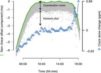
Figure 1 shows an example of a clock skew measurement across the Internet. The target was 22 hops away with an average Round Trip Time (RTT) of 325 ms. The target was a PC with Intel Celeron 2.6 GHz CPU running FreeBSD 4.10, and measurements were taken from the TCP timestamp clock, which has a frequency of 1 kHz. No additional CPU load was generated on the target during the measurement.
The constant clock skew sc has already been removed. The grey dots (·) are the offsets between the two clocks, the green line (-) on top is the piece-wise estimation of the variable skew and the blue triangles (Δ) are the negated values of the derivative of the variable clock skew (the negated clock skew change).
The noise apparent in the figure has two components: the network jitter (on the path from the target to the attacker) and the quantisation error. Note that the network jitter also contains noise inherent in measuring when packets are received by the attacker, and noise caused by variable delay at the target between generating the timestamps and sending packets. In Figure 1 , we can clearly see the 1 ms quantisation noise band below the estimated slope, caused by the target’s 1 kHz clock. Offsets below this band were also affected by network jitter.
The samples close to the slope on top are the samples obtained immediately after a clock tick (with negligible network jitter). The samples at the bottom of the quantisation noise band are samples obtained immediately before the clock tick. With the linear programming algorithm, only the samples close to the slope on top contribute to the accuracy of the measurement. Assuming an uncongested network, the network jitter is skewed towards zero and small even on long-distance links (see Figure 9). The quantisation noise is inversely proportional to frequency of the target’s clock. Depending on the source of timestamps used and the target’s operating system, the clock frequency is typically between 1 Hz and 1 kHz (resulting in a noise band between 1 s and 1 ms). If the target does not expose a high-frequency clock, the quantisation noise can be significantly larger than the noise caused by network jitter.
To increase the accuracy of the measurement in the presence of high quantisation noise, w must be set to larger values, as the probability of getting samples close to the slope on top increases with the number of samples. However, large w only allow very coarse measurements. Oversampling provides more fine-grained results while keeping w large to minimise the error. Without oversampling the time windows do not overlap and the start times of windows are S = {0,w,2w,…,nw}. With oversampling, the windows overlap and hence the windows start at times S = {0,w∕o,2w∕o,…,nw∕o}, where o is the oversample factor.
However, even with large values of w, over-sampling has a number of drawbacks. The first estimate is obtained after w∕2 (regardless of o), meaning that for large w it is impossible to get estimates close to the start and end of measurements. Furthermore, large w make it impossible to accurately measure steep clock-skew changes. For example, such changes happen when a CPU load inducement is started and the temperature increases quickly [3]. Another disadvantage of oversampling is the increased computational complexity of O(o·n·w) compared to O(n·w) without over-sampling to obtain the same number of clock skew estimates per time interval.
Previous research used different timestamps sources for clock-skew estimation: ICMP timestamp responses, TCP timestamp header extensions or TCP sequence numbers [4, 3].
TCP sequence numbers on Linux are the sum of a cryptographic result and a 1 MHz clock. They provide good clock-skew estimates over short periods because of the high frequency, but re-keying of the cryptographic function every five minutes makes longer measurements non-trivial [3].
ICMP timestamps have a fixed frequency of 1 kHz. Their disadvantage is that they are affected by clock adjustments done by the Network Time Protocol (NTP) [9], which makes estimation of variable clock skew more difficult. Furthermore, ICMP messages are now blocked by many firewalls.
TCP timestamps have a frequency between 1 Hz and 1 kHz, depending on the operating system. Their advantage is that they are generated before NTP adjustments are made [4]. TCP timestamps are currently the best option for clock-skew measurement because they are widely available and unaffected by NTP (at least for Linux, FreeBSD and Windows [4]). However, even TCP timestamps are not available in all situations. They may not be enabled on certain operating systems and they cannot be used if there is no end-to-end TCP connection to the target. For example, they cannot be used through the Tor anonymisation network.
HTTP timestamps have a frequency of 1 Hz and are available from every web server. However, these have not been previously used for clock-skew measurement due to the low frequency. We describe how to exploit them in the following section.
A major disadvantage of the attack in [3] is that the attacker needs to exchange large amounts of traffic with the hidden service across the Tor network in order to accurately measure clock skew changes. It may not be possible to actually send sufficient traffic because Tor does not provide enough bandwidth, or because the service operator actively limits the request rate to avoid overload, prevent Denial of Service (DoS) attacks etc. Furthermore, the attack also relies on an exposed high-frequency timestamp source (experiments used the 1 kHz TCP timestamp) on the target for adequate clock-skew estimation.
The synchronised sampling technique proposed in this paper improves the existing attack reducing the duration and amount of network traffic required. Measuring clock-skew requires only a small amount of traffic compared to the amount of traffic needed for load inducement. For example, the exchange of one request/response every 1.5 s is sufficient for clock-skew estimation.
Our improvements also make the existing attack applicable in situations where high-resolution timestamps are not available. For example ICMP or TCP timestamps (see Section 3.1) are not available across Tor, since it only supports TCP and streams are re-assembled on the client, removing any headers. Because our proposed technique allows accurate clock-skew estimation from low-resolution timestamps, HTTP timestamps obtained from a hidden web server across the Tor network could be used. The fact that low-resolution timestamps are usable opens the door to new variants of the attack.
In the first new attack variant, the attacker measures the variable clock skew of the hidden service via Tor, and of all the candidate hosts via accessing the IP addresses directly. Then the attacker compares the variable clock-skew pattern of the hidden service with the patterns of all the candidates. The variable clock skew patterns of different hosts differ sufficiently over time, and the duration of the attack could be increased arbitrarily. While this attack has the benefit of not requiring large amounts of traffic to be exchanged, it could still take a long time. The attacker must ensure that both timestamp sources are derived from the same physical source
A quicker version of this attack could only compare the fixed clock-skew of the target measured via Tor with the fixed clock-skew measured directly for all candidates. Kohno et al. showed that clock skew of a particular host changes very little over time, but the difference between different hosts is significant [4].
Another new attack variant is based on the idea of using clock-skew estimates for geo-location [3]. The attacker identifies the location of the candidates based on their IP addresses and a geo-location database. For example, GeoLite is a freely available database that maps IP addresses to locations with a claimed accuracy of over 98% [10]. The attacker measures the variable clock skew of the hidden service via Tor. The attacker then estimates the location based on the variable clock-skew pattern using the technique described in [3].
This attack works even in cases where the attacker cannot access the candidate hosts directly. On the other hand this attack does not allow an unambiguous identification of the hidden service if candidate locations are geographically close together.
The key common factor among the new attacks discussed above is that clock skew must be estimated from responses sent over the hidden service channel. Previous work has not examined this option because typically only a low frequency clock is available and quantisation noise dominates the small effect of temperature on clock skew. However, in this paper we will show how it is still possible to exploit this clock. Here, the attacker acts as HTTP client sending minimal HTTP requests to the target. Standard web servers include a 1 Hz timestamp in the Date header of HTTP responses because it was recommended for HTTP 1.0 [11] and is mandatory for HTTP 1.1 (excluding 5xx server errors and some 1xx responses) [12].
Before the HTTP exchange a TCP connection needs to be established between client and server. Including TCP connection establishment, it may take at least two full round trip times from when the client wants to send a request until the response is received. To minimise the TCP overhead, the client should open a TCP connection beforehand. Ideally, it should only open the connection once and then keep it alive for the duration of the measurement. However, it is not possible for a client to force a server to keep a connection open. Therefore, when the client notices that the server has closed the connection, it should immediately re-open it. Then, the next HTTP request can be sent at the appropriate time determined by the synchronised sampling algorithm.
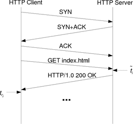
The HTTP timestamp is usually generated after the server has received the client’s request. We verified that Apache 2.2.x generates the timestamp after the request has been successfully parsed [13]. The corresponding client timestamp is the time the packet containing the Date header is received, which is usually the first packet sent by the server after the TCP connection has been fully established (see Figure 2).
Previous approaches to remote clock-skew estimation have sampled timestamps at random times. However, with the 1 Hz HTTP timestamp, the consequent high quantisation noise would prevent the attack from accurately measuring the target’s clock skew within a feasible period. Instead, we must probe the target’s clock immediately after a clock tick occurred, because here the quantisation error is the smallest. To achieve this, the attacker has to synchronise its probing phase and frequency such that probes arrive shortly after the clock tick. We assume the attacker selects a nominal sample frequency, based on the desired accuracy and intrusiveness of the measurement.
The attacker cannot measure the exact time difference between the arrival of probe packets and the clock ticks. To maintain synchronisation, the attacker has to alternate between sampling before and after the clock tick. Samples before the clock tick can be corrected by adding one tick, as their true value is actually closer to the next clock tick. However, the linear programming algorithm still cannot use these samples because for them the quantisation error and jitter are in opposite directions and cannot be separated.
Figure 3 illustrates the benefit of synchronised sampling over random sampling. The solid step line is the target’s clock value over time and the dashed line shows the true time. Random samples are distributed uniformly between clock ticks whereas synchronised samples are taken close to the clock ticks. Note that in the figure, the time for samples before the tick has been corrected as described above. The quantisation errors are the differences between samples’ y-values and the true time. The absolute quantisation errors are shown as bars at the bottom. Synchronised sampling leads to smaller errors in comparison with random sampling.
Our algorithm is similar to existing Phase Lock Loop (PLL) techniques used for aligning the frequency and phase of a signal with a reference [14]. However, whereas PLL techniques measured the phase difference of two signals, we can only estimate the phase difference by detecting whether a sample was taken before or after the clock tick.
Initially, the attacker starts probing with the nominal sample frequency and measures how many clock ticks occur in one sample interval (target_ticks_per_interval). The measurement is repeated to obtain the correct number of ticks.
The attacker cannot measure the exact time difference between the arrival of a probe packet and the target’s clock tick. However, the attacker can measure the position of the probe arrival relative to the target’s clock tick based on the number of clock ticks that occurred between the current and the last timestamp of the target (ticks_diff ). If the number of clock ticks is less than target_ticks_per_interval, the sample was taken before the tick and vice versa. If ticks_diff equals target_ticks_per_interval the position is left unchanged. At the start of the measurement the position is not known and the attacker needs to continuously increase or decrease the probe interval until a change occurs (initial phase lock).
The probe interval (the reciprocal of the probe frequency) is controlled using the following mechanism (see Algorithm 1). The probe interval is adjusted based on the position errors each time a position change occurs and the previous position was known using a Proportional Integral Derivative (PID) controller [15]. PID controllers base the adjustment not only on the last error value, but also on the magnitude and the duration of the error (integral part) as well as the slope of the error over time (derivative part). Kp, Ki and Kd are pre-defined constants of the PID controller.
Alternatively, the linear programming algorithm [8] could be used to compute the relative clock skew between attacker and target based on a sliding window of timestamps. The probe interval is then adjusted based on the estimated relative clock skew. This technique works well if the estimates are fairly accurate, which is the case for high-frequency clocks and low network jitter.
|
In order to maintain the synchronisation, the attacker has to enforce regular position changes. This is done by modifying the time the next probe is sent. If the current position is before the clock tick the send time of the next probe is increased based on the last adjustment last_adj_before. If the current position is behind the clock tick the next probe send time is decreased based on the last adjustment last_adj_behind. The adjustments are modified based on how well the attacker is synchronised to the target.
If a change of position occurs between two samples, the difference between the arrival of the probe packet and the target’s clock tick is smaller than the last adjustment and therefore the next adjustment is decreased. If no position change occurs the error is assumed to be larger than the last adjustment and the next adjustment is increased. The initial probe send-time adjustment is a pre-defined constant. Algorithm 2 shows the probe send time adjustment algorithm. α and β are pre-defined constants that determine how quickly the algorithm reacts (0 < α < 1 and β > 1).
|
The probe frequency and send time adjustments are limited to a range between pre-defined minimum and maximum values to avoid very small or very large changes.
Loss of responses is detected using sequence numbers. A sequence number is embedded into each probe packet such that the target will return the sequence number in the corresponding response. The actual field depends on the protocol used for probing. For example, for ICMP the sequence number is the ICMP Identification field whereas for TCP the sequence number is the TCP sequence number field.
For HTTP it is not possible to embed a sequence number directly into the protocol. Instead, sequence numbers are realised by making requests cycling through a set of URLs. A sequence number is associated with each URL and HTTP responses are mapped to HTTP requests using the content length assumed to be known for each object. This technique assumes there are multiple objects with different content lengths accessible on the web server.
If packet loss is detected, the algorithm adjusts ticks_diff by subtracting the number of lost packet multiplied by target_ticks_per_interval. Reordered packets are considered lost.
Algorithm 3 shows the synchronisation procedure. Our algorithm works with different timestamps and different clock frequencies. It has been tested with ICMP, TCP and HTTP timestamps and TCP clock frequencies of 100 Hz, 250 Hz and 1 kHz.
|
Any constant delay does not affect the synchronisation process. However, changes in delay on the path from the attacker to the target will affect the arrival time of the probe packets. This could be caused by jitter in the sending process (jitter inside the attacker), network jitter (queuing delays in routers) or jitter in the target’s packet receiving process.
Often we can assume the network is uncongested and therefore network jitter is skewed towards zero. This is usually the case in a LAN (see Section 6). Even on the Internet many links are not heavily utilised and path changes (caused by routing changes) are usually infrequent. Load-balancing is usually performed on a per-flow basis to eliminate any negative impacts on TCP and UDP performance.
However, when measuring clock skew over a Tor circuit we expect much higher network jitter. A Tor circuit is composed of a number of network connections between different nodes. The overall jitter does not only include the jitter of each connection but also the jitter introduced by the Tor nodes themselves.
The timing of sending probes is not very exact if the sender is a userspace application. Even if the userspace send() system call is called at the appropriate time, there will be a delay before the packet is actually sent onto the physical medium. The variable part of this delay can cause probe packets to arrive too late or too early. This error could be reduced by running the software entirely in the kernel (e.g. as kernel module), using a real-time operating system or by using special network cards supporting very precise sending of packets. Any variable delay in the packet receiving process of the target has the same effect and is unfortunately out of control of the attacker. The only way an attacker could reduce such errors would be to adjust the sending of the probe packets based on a prediction of the jitter inside the target, which appears to be a challenging task.
Another error is introduced when the relative clock skew between attacker and target changes and the algorithms needs to adjust the probe frequency. The attacker is able to control its time keeping and avoid any sudden clock changes. But if the target is running NTP and the timestamps are affected by NTP adjustments, changes in relative clock skew are possible.
In the first part of this section we compare the accuracy of synchronised and random sampling in a LAN testbed using TCP timestamps with typical target clock frequencies of 100 Hz, 250 Hz and 1000 Hz, as well as 1 Hz HTTP timestamps. Since in the LAN network jitter is negligible the results show the maximum improvement of using synchronised sampling and demonstrate that our implementation is working correctly.
In the second part we compare the accuracy of synchronised and random sampling based on TCP timestamps across a 22-hop Internet path. The result shows that even on a long path, synchronised sampling significantly increases clock-skew estimation accuracy, which improves on the attack proposed by Murdoch [3].
In the third part we compare the accuracy of synchronised and random sampling for probing a web server running as a Tor hidden service. We show that synchronised sampling improves clock skew estimation significantly, even over a path with high network jitter. We also show that a hidden web sever can be identified among a candidate set by comparing the variable clock skew over time using synchronised sampling. Furthermore, using synchronised sampling shows daily temperature patterns that could not be identified using random sampling.
Finally, we investigate how long our technique needs for the initial synchronisation (the time until the attacker has locked on to the phase and frequency of the target’s clock ticks). We compare the times for HTTP probing in a LAN and probing a hidden web server over a Tor network.
To evaluate the accuracy of synchronised and random sampling we need to know the true values of the variable clock skew. Since it is impossible to directly measure this, we use the following approach. In our tests the target also runs a UDP server and the attacker runs a UDP client. The UDP client sends requests to the server at regular time intervals. Upon receiving a request, the UDP server returns a packet with a timestamp set to the send time of the response. The UDP client records the time it receives the response.
We compute the offset between the two timestamp-series and estimate the variable clock skew as usual. Since the UDP-based timestamp has a precision of 1 μs, the quantisation error is negligible. Although these UDP estimates are not the true values of the variable clock skew we use them as baseline for synchronised and random sampling, which have much higher quantisation errors. In the following we refer to this as UDP probing or UDP measurement.
A drawback of our current implementation is that the UDP server is a userspace program. The server’s response timestamp is taken in userspace before the response packet is sent via the sendto() system call. To reduce these timing errors one could implement a kernel-based version of the UDP server.
We compare the variable skew estimates for
synchronised and random sampling with the reference values, from
the UDP measurement, using the root mean square error (RMSE) of
the data values x against the
reference values  :
:
|
(2) |
We also compute histograms of the noise band for synchronised and random sampling. The noise is defined as difference between the variable clock offset and the UDP timestamp estimated variable skew. For random sampling the quantisation noise band is always uniform with width 1∕f , where f is the clock frequency. For synchronised sampling the quantisation noise depends on how well the synchronised sampling algorithm is able to track the target’s clock tick. For synchronised sampling the noise is given by the samples taken after the clock tick because only these samples are used to estimate the clock skew.
In all experiments we set α = 0.5 and β = 1.5. For TCP timestamps the linear programming algorithm was used to adjust the probe interval with a sliding window of size 120 (LAN) and 300 (Internet). For HTTP timestamp measurements the probe interval was adjusted using the PID controller with Kp = 0.09, Ki = 0.0026 and Kd = 0.02.
The attacker was a PC with Intel Xeon 3.6 GHz Quad-Core CPU running Linux 2.6. The target was a PC with Intel Xeon 3.6 GHz Quad-Core CPU running Linux 2.6 with a TCP timestamp frequency of 1 kHz. Attacker and target were connected to the same Ethernet switch. The attacker simultaneously performed synchronised, random and UDP probing. Synchronised and random probing had an average sampling period of 1.5 s, the same rate as in [3]. The UDP probing was performed with a faster sample rate of 1 s in order to achieve a higher accuracy for the reference measurement. A second UDP measurement with an average sample rate of 1 s was run in order to investigate the error between UDP measurements. The duration of the test was approximately 24 hours.
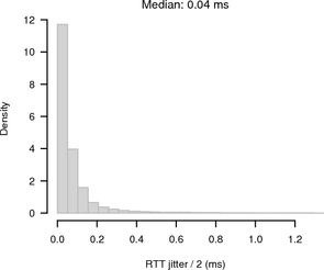
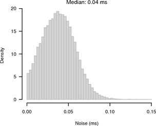
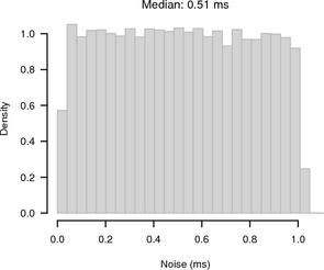
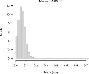
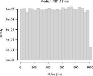
As the test was run inside a LAN the average RTT was only 130 μs and the RTT / 2 jitter was small with a maximum of 60 μs and a median of 30 μs. Figure 4 shows histograms of the noise bands of synchronised and random sampling with respect to the reference given by the UDP measurement. For synchronised sampling most of the offsets are within 100 μs whereas for random sampling we see the expected 1 ms noise band.
|
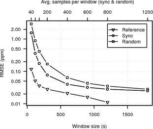
In Figure 5 we compare the RMSE of synchronised sampling, random sampling and the second UDP measurement for different window sizes against the UDP reference with maximum window size (1800 s). We also compare the UDP reference against itself at smaller window sizes. The oversampling factor was chosen such that the time between two clock-skew estimates is the same regardless of the window size (30 s). This has the advantage of providing approximately the same number of estimates for all window sizes. (For smaller window sizes there are still more samples, because there are samples closer to the start and end of the measurement period.)
|
Figure 5 shows that synchronised sampling performs significantly better than random sampling. There is a difference between the second UDP measurement and the UDP reference, but it is smaller than the difference between synchronised sampling and the UDP reference for all window sizes. Hence we conclude the error of UDP measurements is sufficiently small for using it as baseline. In the later experiments we performed only one UDP measurement.
The target clock frequency was 1 kHz, which is the maximum TCP timestamp frequency of current operating systems. However, it is likely that in reality many hosts actually have lower TCP clock frequencies. For example, 100 Hz is the clock frequency used by older Linux and FreeBSD kernels and 250 Hz is the clock frequency of modern Linux 2.6 kernels.
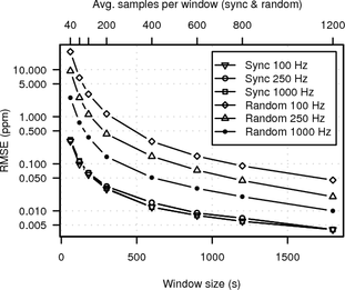
To evaluate the RMSE for lower clock frequencies we used the same setup. This time we ran three synchronised and three random probing processes simultaneously for 24 hours, rounding the target timestamps so that we effectively measured 100 Hz, 250 Hz and 1 kHz clocks. Figure 6 shows the RMSE for synchronised and random sampling for the different target clock frequencies. The UDP measurement has been omitted for better readability. The graph shows that the accuracy of synchronised sampling does not depend on the clock frequency and the RMSE for random sampling increases significantly for lower clock frequencies.
|
In another LAN experiment we ran a web server (Apache 2.2.4) on the target and the attacker used HTTP probing. The average sampling interval was 2 s, because this is the minimum probe frequency for 1 Hz HTTP timestamps. The web server was completely idle (except for the requests generated by the attacker). The duration of the experiment was approximately 24 hours.
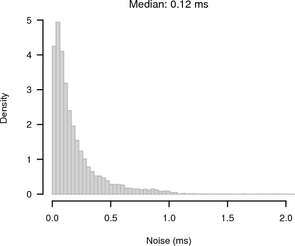
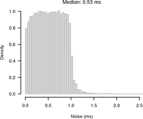
Although the experiment was carried out between the same two hosts as before, the RTT / 2 jitter was higher with a maximum of 120 μs and a median of 60 μs. The web server running in userspace introduced the additional jitter. Figure 7 shows the noise for synchronised sampling and random sampling. For synchronised sampling the noise band is only slightly larger than in Figure 4. Because of the higher jitter, the synchronisation is less accurate. For random sampling the noise band is 1 s because of the 1 Hz HTTP clock frequency.
|
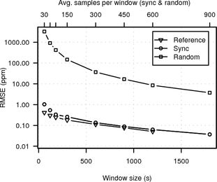
Figure 8 shows the RMSE of synchronised sampling, random sampling and the UDP measurement against the reference at maximum window size. The RMSEs of synchronised sampling and UDP reference are very similar to the results in Figure 5. Because of the large noise band, the RMSE for random sampling is more than two orders of magnitude above the RMSE for synchronised sampling. This demonstrates that our new algorithm is able to effectively measure clock skew changes for low frequency clocks, an infeasible task for random sampling.
|
|
The attacker was the same machine as in Section 6.1 located in Cambridge, UK. The target was 22 hops away located in Canberra, Australia. The target was a FreeBSD 4.10 PC with a kernel tick rate set to 1000 and therefore the TCP timestamp frequency was 1 kHz. The average RTT between measurer and target was 325 ms. The duration of the measurement was approximately 21 hours. We performed synchronised, random and UDP probing.
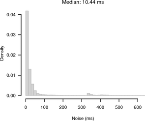
Despite the high RTT, the jitter is small and skewed towards zero as shown in Figure 9.
Figure 10 shows histograms of the noise bands of synchronised and random sampling in relation to the reference given by the UDP measurement. For synchronised sampling most of the offsets are within 250 μs of the reference whereas for random sampling there is the expected 1 ms noise band.
|
Figure 11 shows the RMSE of synchronised sampling, random sampling and the UDP reference against the UDP reference at maximum window size using the same parameters as in Section 6.1. The gain of synchronised sampling is smaller compared to Section 6.1 because of the higher network jitter but still significant for smaller window sizes.
|
For our measurements we used a private Tor network. Our Tor nodes are distributed across the Internet running on Planetlab [16] nodes. The main reason for using a private Tor network instead of the public Tor network is the poor performance of hidden services in the public Tor network. Besides huge network jitter that prevents any accurate clock-skew measurements, hidden services always disappeared after few hours preventing longer measurements. While currently it is difficult to carry out the attack in the public Tor network, it should become easier in the future, as the Tor team is now working on improving the performance of hidden services.
We selected 18 Planetlab widely geographically distributed nodes on which we ran Tor nodes (of which 3 were directory authorities). We selected nodes that had low CPU utilisation at the time of selection. An Intel Core2 2.4 GHz with 4 GB RAM running Linux 2.6.16 was used to run another Tor node and the hidden web server. No load is induced on the server, so any clock skew changes are based on the ambient temperature changes.
An Intel Celeron 2.4 GHz with 1.2 GB of RAM running Linux 2.6.16 was used to run a Tor client and our probe tool. We used tsocks [17] with the latest Tor related patches to enable our tool to interact with the Tor client via the SOCKS protocol and to properly handle Tor hidden server pseudonyms.
First we performed an experiment similar to the ones in Section 6.1 and Section 6.2. Synchronised and random sampling was performed across the Tor network, while UDP probing was performed directly between the client machine and the hidden server. The measurement duration was approximately 18 hours.
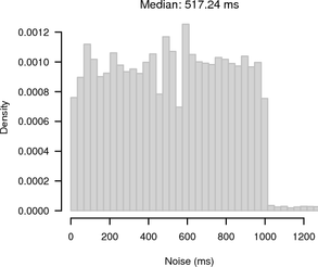
The average RTT between client and hidden server across Tor was 885 ms. Figure 12 shows the RTT / 2 jitter, which is considerably higher than in the previous measurements.
|
|
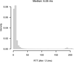
Figure 13 shows histograms of the noise bands of synchronised and random sampling. For random sampling it shows the expected 1 s noise band. For synchronised sampling the noise is greatly reduced. Most of the offsets are ≤ 100 ms away from the slope given by the UDP reference.
|
|
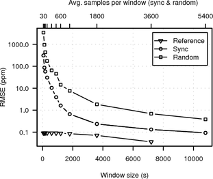
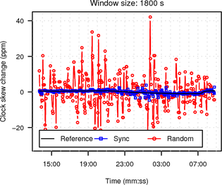
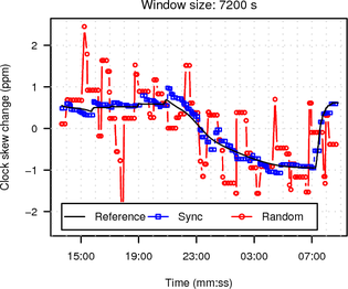
In Figure 15 we compare the RMSE of synchronised sampling, random sampling and the UDP reference against the UDP reference at maximum window size. The RMSE of synchronised sampling is almost one magnitude lower than the RMSE for random sampling even for window sizes as large as two hours.
|
In the second experiment we performed the actual attack. We treated all 19 Tor nodes as candidates and measured their clock skew directly using TCP timestamps (synchronised sampling). At the same time we measured the clock skew of the hidden web service via Tor based on HTTP timestamps using synchronised and random sampling simultaneously. The experiment lasted about ten hours. One of the nodes stopped responding in the middle of the experiment.
Figure 16 shows the RMSE of the HTTP clock skew estimates obtained from the hidden service via Tor using random sampling or synchronised sampling and TCP clock skew estimates of all candidate nodes. We used a window size of three hours and set the oversample factor so one clock estimate is obtained every 30 s. (For smaller windows random sampling was not able to consistently select one candidate as the best and would alternate between a few including the correct one for the whole duration of the measurement.)
 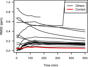
|
The RMSE of the HTTP timestamp estimate and the correct candidate is shown as thick grey (red on colour display) line while RMSEs for all other candidates are shown as thin black lines.
The RMSE between the synchronised sampling Tor measurement and the direct measurement of the correct candidate is very small, and with increasing duration becomes significantly smaller than the RMSE of the Tor measurement and all the other candidates except one. For random sampling all RMSEs are fairly high indicating that there is no good match of the variable clock skew of the Tor hidden service with any of the candidates. In the second half of the experiment the RMSE of the correct candidate becomes smallest, but only by a very small margin.
Synchronised sampling is able to identify the correct candidate much faster than random sampling, needing only 139 minutes compared to 287 minutes. These times are from the start of the measurement until the RMSE of the correct candidate becomes smallest. They include the initial 1.5 hours it takes to get the first clock skew estimate (because of the three hour windows), which is not included in Figure 16.
While the variable clock skew of the TCP clock and userspace clock (HTTP timestamps) are a good match the fixed skew of the two clocks differs on our Linux 2.6.16 box running the hidden server. This makes it impossible to evaluate an identification of the hidden server based on the fixed skew. However, since we know the true fixed skew of the userspace clock, we can analyse how long it takes to get an estimate using synchronised and random sampling of the HTTP clock. We use the data from the previous measurement and assume the skew estimate is correct if within 0.5 parts per million of the true value. Again synchronised sampling outperforms random sampling, needing only 23 minutes compared to 102 minutes.
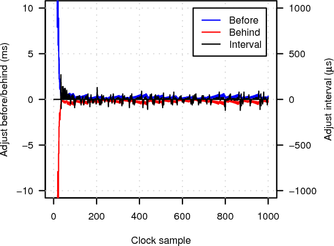
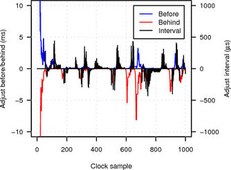
We briefly analyse the initial synchronisation time of our technique. The initial synchronisation is the time it takes until the attacker has locked on to the phase and frequency of the target’s clock ticks.
Figure 17 plots the values of adj_before, adj_behind and probe_interval (see Section 5 for the meaning of the variables) over the number of clock samples (taken from the target’s clock every 2 s). The y-axis range is limited to between -10 ms and 10 ms and the x-axis is limited to the first 1000 clock samples. Note that before adjustments are always positive, while behind adjustments are always negative.
|
In the LAN experiment initial synchronisation is established after only about 40 samples (roughly 1.5 minutes) and further adjustments and probe interval changes are small (less than 500 μs and 100 μs respectively). When probing over the Tor network synchronisation is more difficult because of the much higher network jitter. Consequently initial synchronisation takes longer (about 70 clock samples or roughly 2.5 minutes) and the algorithm is forced to make larger adjustments and probe interval changes (of up to several milliseconds).
In this paper we have presented and evaluated an improved technique for remote clock-skew estimation based on the idea of synchronised sampling proposed by Murdoch [3]. The evaluation shows that our new algorithm provides more accurate clock skew estimates than the previous random sampling based approach. Especially if the target clock frequency is low, accuracy improves by up to two orders of magnitude. Since the accuracy of our synchronised sampling technique is independent of the target’s clock frequency, it is possible to estimate variable clock-skew from low-resolution timestamps.
Our technique does not only improve the previously proposed clock-skew related attack on Tor [3], it also opens the door for new variants of the attack, which we have described in the paper. Our technique could also be used to improve the identification of hosts based on their clock skew as proposed in [4] if active measurement is possible.
Currently our Tor test network is fairly small and only has one hidden server. While we showed that our new proposed attacks work in principle, we did not provide a comprehensive evaluation. In future work we plan to extend our test network and add more hidden servers. This will allow us to perform a more detailed evaluation including analysing the sensitivity and specificity of our attack based on the different parameters.
The synchronised sampling implementation could be further improved by fine-tuning the algorithm parameters. Our current implementation runs in userspace, which naturally limits the ability to exactly time probe packets. A kernel implementation, using network cards capable of high-precision traffic generation, or use of a real-time kernel, could achieve higher accuracy.
We thank Markus Kuhn and the anonymous reviewers for their valuable comments.
[1] P. Syverson R. Dingledine, N. Mathewson. Tor: The second-generation onion router. In Proceedings of the 13th USENIX Security Symposium, August 2004.
[2] Reporters Without Borders. Blogger and documentary filmmaker held for the past month, March 2006. https://www.rsf.org/article.php3?id_article=16810.
[3] S. J. Murdoch. Hot or not: Revealing hidden services by their clock skew. In CCS ’06: Proceedings of the 9th ACM Conference on Computer and Communications Security, pages 27—36, Alexandria, VA, US, October 2006. ACM Press.
[4] T. Kohno, A. Broido, and kc claffy. Remote physical device fingerprinting. In Proceedings of IEEE Symposium on Security and Privacy, pages 211—225, May 2005.
[5] David M. Goldschlag, Michael G. Reed, and Paul F. Syverson. Onion routing. Communications of the ACM, 42(2):39—41, February 1999.
[6] Lasse Øverlier and Paul F. Syverson. Locating hidden servers. In IEEE Symposium on Security and Privacy, pages 100—114, Oakland, CA, US, May 2006. IEEE Computer Society.
[7] Steven J. Murdoch and George Danezis. Low-cost traffic analysis of Tor. In IEEE Symposium on Security and Privacy, pages 183—195, Oakland, CA, US, May 2005. IEEE Computer Society.
[8] D. Towsley S. B. Moon, P. Kelly. Estimation and removal of clock skew from network delay measurements. Technical Report 98-43, Department of Computer Science, University of Massachussetts at Amherst, October 1998.
[9] D. Mills. Network Time Protocol (Version 3) Specification, Implementation. rfc 1305, IETF, March 1992. https://www.ietf.org/rfc/rfc1305.txt.
[10] MaxMind. GeoLite Country, 2008. https://www.maxmind.com/app/geoip_country.
[11] T. Berners-Lee, R. Fielding, and H. Frystyk. Hypertext Transfer Protocol — HTTP/1.0. rfc 1945, IETF, May 1996. https://www.ietf.org/rfc/rfc1945.txt.
[12] R. Fielding, J. Gettys, J. Mogul, H. Frystyk, L. Masinter, P. Leach, and T. Berners-Lee. Hypertext Transfer Protocol — HTTP/1.1. rfc 2616, IETF, June 1999. https://www.ietf.org/rfc/rfc2616.txt.
[13] Apache Software Foundation. Apache web server. https://www.apache.org/.
[14] C. Langton. Unlocking the phase lock loop - part 1, 2002. https://www.complextoreal.com/chapters/pll.pdf.
[15] Carnegie Mellon University. Pid tutorial. https://www.engin.umich.edu/group/ctm/PID/PID.html.
[16] Brent Chun, David Culler, Timothy Roscoe, Andy Bavier, Larry Peterson, Mike Wawrzoniak, and Mic Bowman. PlanetLab: An overlay testbed for broad-coverage services. ACM SIGCOMM Computer Communication Review, 33(3), July 2003.
[17] S. Clowes. Tsocks - a transparent socks proxying library. https://tsocks.sourceforge.net/.