Mahmut Kandemir, Seung Woo Son
Department of Computer Science and Engineering
The Pennsylvania State University
Mustafa Karakoy
Department of Computing
Imperial College
This paper presents a compiler-directed code restructuring scheme for improving the I/O performance of data-intensive scientific applications. The proposed approach improves I/O performance by reducing the number of disk accesses through a new concept called disk reuse maximization. In this context, disk reuse refers to reusing the data in a given set of disks as much as possible before moving to other disks. Our compiler-based approach restructures application code, with the help of a polyhedral tool, such that disk reuse is maximized to the extent allowed by intrinsic data dependencies in the application code. The proposed optimization can be applied to each loop nest individually or to the entire application code. The experiments show that the average I/O improvements brought by the loop nest based version of our approach are 9.0% and 2.7%, over the original application codes and the codes optimized using conventional schemes, respectively. Further, the average improvements obtained when our approach is applied to the entire application code are 15.0% and 13.5%, over the original application codes and the codes optimized using conventional schemes, respectively. This paper also discusses how careful file layout selection helps to improve our performance gains, and how our proposed approach can be extended to work with parallel applications.
In the recent past, large scale applications in science and engineering have grown dramatically in complexity. As a result, scientists and engineers expend great effort to implement software systems that carry out these applications and interface them with the instruments and sensors that generate data. Apart from their huge computational needs, these large applications have tremendous I/O requirements as well. In fact, many scientific simulations tend to generate huge amounts of data that must be stored, mined, analyzed, and evaluated. For example, in a combustion application [39], features based on flame characteristics must be detected and tracked over time. Based upon evolution, simulations need to be steered in different regions, and different types of data need to be stored for further analysis. A simulation involving three-dimensional turbulent flames involving detailed chemistry can easily result in 5 tera-bytes of data being stored on disk, and the total storage requirement can be in the order of peta-bytes when one considers the fact that numerous such simulations have to be performed to reach meaningful and accurate conclusions. Other scientific applications have also similar storage and I/O requirements.
Unfortunately, as far as software - in particular compilers - are concerned, I/O has always been neglected and received much less attention in the past compared to other contributors to an application's execution time, like CPU computation, memory accesses and inter-CPU communication. This presents an important problem, not just because modern large-scale applications have huge I/O needs, but also the progresses in storage hardware are not in the scale that can meet these pressing I/O demands. Advances in disk technology have enabled the migration of disk units to 3.5-inch and smaller diameters. In addition, the storage density of disks has grown at an impressive 60 percent annually, historically, and has accelerated to greater than a 100 percent rate since 1999 [20]. Unfortunately, disk performance has not kept pace with the growth in disk capacities. As a result, I/O accesses are among primary bottlenecks in many large applications that store and manipulate large data sets. Overall, huge increases in data set sizes combined with slow improvements in disk access latencies motivate for software-level solutions to the I/O problem. Clearly, this I/O problem is most pressing in the context of data-intensive scientific applications, where increasingly larger data sets are processed.
While there are several ways of improving I/O behavior of a large application, one of the promising approaches has been cutting the number of times the disks are accessed during execution. This can be achieved at different layers of the I/O subsystem and be attacked by using caching which keeps frequently used data in memory (instead of disks) or by restructuring the application code in a way that maximizes data reuse. While both the approaches have been explored in the past [2,3,9,10,16,21,24], the severity of the I/O problem discussed above demands further research. In this paper, we focus on a compiler-directed code restructuring for improving I/O performance of large-scale scientific applications that process disk-resident data sets. A unique advantage of the compiler is that it can analyze an entire application code, understand global (application wide) data and disk access patterns (if data-to-disk mapping is made available to it), and - based on this understanding - restructure the application code and/or data layout to achieve the desired performance goal. This is a distinct advantage over pure operating system (OS) based approaches that employ rigid, application agnostic optimization policies as well as over pure hardware based techniques that do not have the global (application wide) data access pattern information. However, our compiler based approach can also be used along with OS and hardware based schemes, and in fact, we believe that this is necessary to reach a holistic solution to the growing I/O problem.
The work presented in this paper is different from prior studies that explore compiler support for I/O in at least two aspects. First, our approach can optimize the entire program code rather than individual, parallel loop-nests, as has been the case with the prior efforts. That is, as against to most of the prior work on compiler-directed I/O optimization, which restructure loops independent of each other, our approach can restructure the entire application code by capturing the interactions among different loop nests. An advantage of this is that our approach does not perform a local (e.g., loop nest based) optimization which is effective for the targeted scope but harmful globally. However, if desired, our approach can be applied to individual loop nests or functions/subprograms independently. Second, we also discuss the importance of file layout optimization and of adapting to parallel execution. These two extensions are important as 1) the results with our layout optimization indicate that additional performance savings (7.0% on average) are possible over the case code re-structuring is used alone, and 2) the results with the multi-CPU extension show that this extension brings 33.3% improvement on average over the single-CPU version.
The proposed approach improves I/O performance by reducing the number of disk accesses through disk reuse maximization. In this context, disk reuse refers to reusing the data in a given set of disks as much as possible before moving to other disks. Our approach restructures the application code, with the help of a polyhedral tool [26], such that disk reuse is maximized to the extent allowed by intrinsic data dependencies in the code. We can summarize the major contributions of this paper as follows:
![]() We present a compiler based disk reuse optimization technique
targeting data intensive scientific applications. The proposed approach
can be applied at the loop nest level or whole
application level.
We present a compiler based disk reuse optimization technique
targeting data intensive scientific applications. The proposed approach
can be applied at the loop nest level or whole
application level.
![]() We discuss how the success of our approach can be increased by
modifying the storage layout of data, and how it can be extended to
work under parallel execution.
We discuss how the success of our approach can be increased by
modifying the storage layout of data, and how it can be extended to
work under parallel execution.
![]() We present an experimental evaluation of the proposed approach
using seven large scientific applications. The results collected so
far indicate that our approach is very successful in maximizing disk
reuse, and this in turn results in large savings in I/O latencies.
More specifically, the average I/O improvements brought by the loop nest based
version of our approach are 9.0% and 2.7%, over the original application
codes and the codes optimized using conventional schemes, respectively.
Further, the average improvements obtained when our approach is applied
to the entire application code are 15.0% and 13.5%, over the original
application codes and the codes optimized using conventional schemes,
respectively.
We present an experimental evaluation of the proposed approach
using seven large scientific applications. The results collected so
far indicate that our approach is very successful in maximizing disk
reuse, and this in turn results in large savings in I/O latencies.
More specifically, the average I/O improvements brought by the loop nest based
version of our approach are 9.0% and 2.7%, over the original application
codes and the codes optimized using conventional schemes, respectively.
Further, the average improvements obtained when our approach is applied
to the entire application code are 15.0% and 13.5%, over the original
application codes and the codes optimized using conventional schemes,
respectively.
The rest of this paper is organized as follows. The next section explains the disk system architecture assumed by our compiler. It also presents the key concepts used in the remainder of the paper. Section 3 gives the mathematical details behind the proposed compiler-based approach. Section 4 discusses how our approach can be extended by taking accounts of the storage layout of data. Section 5 gives an extension to capture the disk access interactions among the threads of a parallel application. An experimental evaluation of our approach and a comparison with the conventional data reuse optimization scheme are presented in Section 6. Section 7 discusses related work and Section 8 concludes the paper by summarizing its main contributions and discussing briefly possible future extensions.
 |
We also assume that a portion of the main memory of the computation node is reserved to serve as buffer (also called cache) for frequently used disk data. If a requested data item is found in this cache, no disk I/O is performed and this can reduce data access latencies significantly. While it is possible to employ several buffer management schemes, the one used in this work operates under the LRU policy which replaces the least recently used stripe when a new block is to be brought in. Selection of the buffer management scheme to employ is orthogonal to the main focus of this paper. It is important to note that all the disks in the system share the same buffer (in the computation node) to cache their data, and thus, effective management of this buffer is very critical. Note also that, in addition to the cache in the computation node, the I/O nodes themselves can also employ caches. Our optimization target in this paper, however, is the performance of the cache in the computation node.
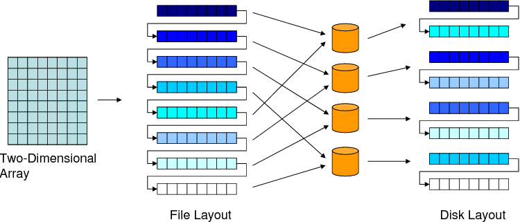 |
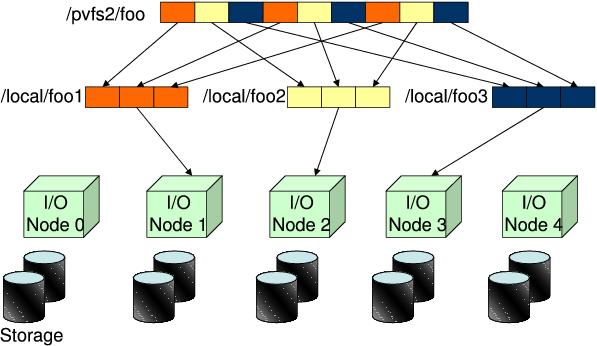
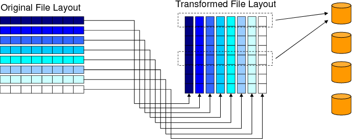
Figure 2 shows the mappings a two-dimensional data array data goes through as far as disk system storage is concerned. Array data in memory is stored in file using some storage order, which may be row-major, column-major, or in a blocked fashion. This is called the file layout. (Note that this may be different from the memory layout adopted by the underlying programming language. For example, a C array can be stored in file using column-major layout as opposed to row-major, which is the default memory layout for multi-dimensional arrays in C.) The file is then striped across the available disks on the system. Therefore, two data elements which are neighbors in the memory space can get mapped to separate disks as a result of this series of mappings. Similarly, data blocks that are far apart from each other can get mapped to the same disk as a result of striping. In this work, when we use the term ``disk-resident array,'' we mean an array that is mapped to the storage system using these mappings. Note that, while it is also possible to map multiple data arrays to one file or one data array to multiple files, in this work we consider only one-to-one mappings between data arrays and files. However, our approach can easily be extended, if desired, to work with one-to-many or many-to-one mappings as well. Unless otherwise stated, all the data arrays mentioned in this paper are disk resident.
 |
Let us now discuss why disk reuse is important and how an optimizing compiler can improve it. The next section gives the technical details of our proposed compiler-based approach to improving disk reuse. Recall that disk reuse means using a data in a given set of disks as much as possible before accessing other disks.
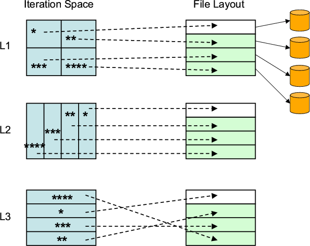
![]() When disk reuse is improved, the chances of finding the requested
data in the buffer increases. As a simple scenario, consider a case in
which a given disk resident array is divided into four stripes and
each stripe is stored on a separate disk. We can expect a very good
buffer performance if the code can be restructured such that accesses
to a given disk are clustered together. This is because such a
clustering improves chances for catching data in the buffer at the
time of reuse. Figure 3 illustrates this scenario. In
this scenario, three different loop nests (L1, L2, and L3) access a
given disk-resident array. Figure 3 shows which portions
of the iteration spaces of these loop nests access what stripes (we
assume 4 stripes). In a default execution, the iteration space can be
traversed in a row-wise fashion. As a result, for example, when the
first row of L1 is executed, two stripes are accessed (and they
compete for the same buffer in the computation node). In our approach
however the iteration spaces are visited in a buffer-aware fashion.
If dependencies allow, we first execute the chunks (marked using *)
from L1, L2, and L3 (one after another). Note that all these chunks
(iterations) use the same stripe (and therefore achieve a very good
data reuse in the buffer). After these, the chunks marked ** are
executed, and these are followed by the chunks marked ***, and so on.
When disk reuse is improved, the chances of finding the requested
data in the buffer increases. As a simple scenario, consider a case in
which a given disk resident array is divided into four stripes and
each stripe is stored on a separate disk. We can expect a very good
buffer performance if the code can be restructured such that accesses
to a given disk are clustered together. This is because such a
clustering improves chances for catching data in the buffer at the
time of reuse. Figure 3 illustrates this scenario. In
this scenario, three different loop nests (L1, L2, and L3) access a
given disk-resident array. Figure 3 shows which portions
of the iteration spaces of these loop nests access what stripes (we
assume 4 stripes). In a default execution, the iteration space can be
traversed in a row-wise fashion. As a result, for example, when the
first row of L1 is executed, two stripes are accessed (and they
compete for the same buffer in the computation node). In our approach
however the iteration spaces are visited in a buffer-aware fashion.
If dependencies allow, we first execute the chunks (marked using *)
from L1, L2, and L3 (one after another). Note that all these chunks
(iterations) use the same stripe (and therefore achieve a very good
data reuse in the buffer). After these, the chunks marked ** are
executed, and these are followed by the chunks marked ***, and so on.
![]() Since our approach clusters disk accesses to a small set of
disks at any given time (and maximizes the number of unused disks), in
a storage system that accommodates power-saving features, unused disks
can be placed into a low-power operating mode
[25,30,40]. However, in this paper we
do not quantify the power benefits of our approach.
Since our approach clusters disk accesses to a small set of
disks at any given time (and maximizes the number of unused disks), in
a storage system that accommodates power-saving features, unused disks
can be placed into a low-power operating mode
[25,30,40]. However, in this paper we
do not quantify the power benefits of our approach.
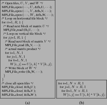
As mentioned earlier, our work focuses on I/O intensive applications that process disk resident arrays. The application codes we target are written in MPI-IO [33], which is the part of the MPI library [12] that handles file I/O related activities. MPI-IO allows synchronous and asynchronous file reads and writes as well as a large set of collective file operations. Figure 4(a) shows an MPI-IO code fragment that performs matrix multiplication on disk resident arrays. For clarity reasons, in our discussion, we omit the MPI-IO commands and represent such a code as shown in Figure 4(b). That is, all the code fragments discussed in this paper are assumed to have the corresponding file I/O commands.
 |
To capture disk accesses and optimize them, we use polyhedral algebra
based on Presburger Arithmetic. Presburger formulas are made of
arithmetic and logic connectives and existential (![]() ) and
universal (
) and
universal (![]() ) quantifiers. In our context, we used them to
capture and enumerate loop iterations that exhibit disk access
locality. We use the term disk map to capture a particular set
of disks (I/O nodes) in the system. For a storage system with
) quantifiers. In our context, we used them to
capture and enumerate loop iterations that exhibit disk access
locality. We use the term disk map to capture a particular set
of disks (I/O nodes) in the system. For a storage system with ![]() disks, we use
disks, we use ![]() =
=
![]() to indicate a disk map. As an example, if
to indicate a disk map. As an example, if ![]() ,
,
![]() = 0110 represents a subset
(of disks) that includes only the second and third disks, whereas 1110
specifies a subset that includes all disks except the last
one. Assuming that array-to-disk mapping (e.g., such as one shown in
Figure 2) is exposed to the compiler, the compiler can set
up a relationship between the loop iterations in an application and
the disks in the storage system the corresponding (accessed) array
elements are stored. For example, if array reference
= 0110 represents a subset
(of disks) that includes only the second and third disks, whereas 1110
specifies a subset that includes all disks except the last
one. Assuming that array-to-disk mapping (e.g., such as one shown in
Figure 2) is exposed to the compiler, the compiler can set
up a relationship between the loop iterations in an application and
the disks in the storage system the corresponding (accessed) array
elements are stored. For example, if array reference ![]() appears
in a loop with iterator
appears
in a loop with iterator ![]() , for a given value of
, for a given value of ![]() we can determine
the disk that stores the corresponding array element (
we can determine
the disk that stores the corresponding array element (![]() ).
).
We define disk locality set as a set of loop iterations - which
may belong to any loop nest in the application code - that access the
set of disks represented by the same disk map. Mathematically, for a
given disk map ![]() , we can define the corresponding disk
locality set (
, we can define the corresponding disk
locality set (
![]() ) as:
) as:
 |
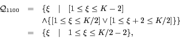
Let us give an example to illustrate the disk locality set concept.
Assume that a disk-resident array ![]() of size
of size ![]() is striped over 4
disks with a stripe of size
is striped over 4
disks with a stripe of size ![]() (i.e., each disk has a single
stripe). Assume further that, for the sake of illustration, we have a
single loop
(i.e., each disk has a single
stripe). Assume further that, for the sake of illustration, we have a
single loop ![]() that iterates from
that iterates from ![]() to
to ![]() and uses two
references,
and uses two
references, ![]() and
and ![]() , to access this disk-resident
array. In this case, we have:
, to access this disk-resident
array. In this case, we have:
An important characteristic of the iterations that belong to the same
![]() is that they exhibit a certain degree of locality
as far as disks are concerned. As a result, if, somehow, we can
transform the application code and execute iterations that belong to
the same
is that they exhibit a certain degree of locality
as far as disks are concerned. As a result, if, somehow, we can
transform the application code and execute iterations that belong to
the same
![]() successively, we can improve disk
reuse (as in the case illustrated in Figure 3). However,
this is not very trivial in practice because of two reasons. First,
the inter-iteration data dependencies in the application code may not
allow such an ordering, i.e., we may not be able to restructure the
code for disk reuse and (at the same time) maintain its original
semantics. Second, even if such an ordering is legal from
the viewpoint of data dependencies, it is not clear how it can be
obtained, i.e., what type of code restructuring can be applied to
obtain the desired ordering. More specifically, it is not clear
whether the transformation (code restructuring) requested for
clustering accesses to a subset of disks can be obtained using a
combination of well-known transformations such as loop fusion, loop
permutation, and iteration space tiling [36]. From a compiler
angle, there is nothing much to do for the first reason. But, for the
second one, polyhedral algebra can be of help, which is investigated
in the rest of the paper.
successively, we can improve disk
reuse (as in the case illustrated in Figure 3). However,
this is not very trivial in practice because of two reasons. First,
the inter-iteration data dependencies in the application code may not
allow such an ordering, i.e., we may not be able to restructure the
code for disk reuse and (at the same time) maintain its original
semantics. Second, even if such an ordering is legal from
the viewpoint of data dependencies, it is not clear how it can be
obtained, i.e., what type of code restructuring can be applied to
obtain the desired ordering. More specifically, it is not clear
whether the transformation (code restructuring) requested for
clustering accesses to a subset of disks can be obtained using a
combination of well-known transformations such as loop fusion, loop
permutation, and iteration space tiling [36]. From a compiler
angle, there is nothing much to do for the first reason. But, for the
second one, polyhedral algebra can be of help, which is investigated
in the rest of the paper.
Suppose, for now, that the application code we have has no dependencies (we will drop this assumption shortly). In this case, we may be able to improve disk reuse (and the performance of the buffer in the computation node) using the following two-step procedure:
![]() For any given
For any given ![]() , execute iterations in the
, execute iterations in the
![]() set consecutively, and
set consecutively, and
![]() In moving from
In moving from
![]() to
to
![]() ,
select
,
select ![]() such that the Hamming Distance between
such that the Hamming Distance between ![]() and
and
![]() is minimum when all possible
is minimum when all possible ![]() s are considered.
s are considered.
The first item above helps us have good disk reuse by executing
the iterations that belong to the subset of disks represented by a
given disk map. The second item, on the other hand, helps us minimize
the number of disks whose status (i.e., being used or not being used)
has to be changed as we move from executing the iterations in
![]() to executing the iterations in
to executing the iterations in
![]() .
As a result, by applying these two rules repeatedly, one can traverse the
entire iteration space in a disk-reuse efficient manner, and this in
turn helps improve the performance of the buffer.
.
As a result, by applying these two rules repeatedly, one can traverse the
entire iteration space in a disk-reuse efficient manner, and this in
turn helps improve the performance of the buffer.
However, real I/O-intensive applications typically have lots of data dependencies and, thus, the simple approach explained above will not suffice in practice. We now discuss how the compiler can capture the dependencies that occur across the different disk locality sets.
We start by observing that the iterations in a given disk locality set
![]() can have data dependencies amongst themselves. We
consider a partitioning (such a partitioning can be obtained using the
Omega library [26] or similar polyhedral tools) of
can have data dependencies amongst themselves. We
consider a partitioning (such a partitioning can be obtained using the
Omega library [26] or similar polyhedral tools) of
![]() into subsets
into subsets
![]() ,
,
![]() ,
, ![]() ,
,
![]() such that
such that
![]() for any
for any ![]() and
and
![]() ,
,
![]() , and for any
, and for any ![]() and
and ![]() ,
all data dependencies are either from
,
all data dependencies are either from
![]() to
to
![]() or from
or from
![]() to
to
![]() . The first two of these constraints indicate that the
subsets are disjoint and collectively cover all the iterations in
. The first two of these constraints indicate that the
subsets are disjoint and collectively cover all the iterations in
![]() , and the last constraint specifies that, as far as
, and the last constraint specifies that, as far as
![]() is concerned, the iterations in any
is concerned, the iterations in any
![]() can be executed successively without any need of
executing an iteration from the set
can be executed successively without any need of
executing an iteration from the set
![]() That is, when we start executing the first iteration
in
That is, when we start executing the first iteration
in
![]() all the remaining iterations in
all the remaining iterations in
![]() can be executed one after another (of course, these
iterations can have dependencies among themselves). We refer to any
such subset
can be executed one after another (of course, these
iterations can have dependencies among themselves). We refer to any
such subset
![]() of
of
![]() as the
``independent disk locality set,'' or the ``independent set'' for short.
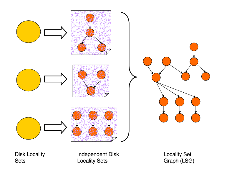
As an example, Figure 5 shows three locality sets (on the
left) and the corresponding independent locality sets (in the
middle). The first locality set in this example contains four
independent locality sets, and these independent locality sets are
connected to each other using three dependence edges. In our approach,
independent locality sets are the building blocks for the main -
graph based - data structure used by the compiler for disk reuse
optimization.
as the
``independent disk locality set,'' or the ``independent set'' for short.
As an example, Figure 5 shows three locality sets (on the
left) and the corresponding independent locality sets (in the
middle). The first locality set in this example contains four
independent locality sets, and these independent locality sets are
connected to each other using three dependence edges. In our approach,
independent locality sets are the building blocks for the main -
graph based - data structure used by the compiler for disk reuse
optimization.
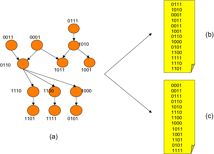
This graph, called the ``locality set graph'' or LSG for short, can be
defined as ![]() =(
=(![]() ,
, ![]() ) where each element of
) where each element of ![]() represents an
independent disk locality set, and the edges in
represents an
independent disk locality set, and the edges in ![]() capture the
dependencies between the elements of
capture the
dependencies between the elements of ![]() . In other words, an LSG has
the
. In other words, an LSG has
the
![]() sets as its nodes and the dependencies
among them as its edges. The right portion of Figure 5
shows an example LSG. The question then is to schedule the nodes of
the LSG while preserving the data dependency constraints between the
nodes. What we mean by ``scheduling'' in this context is determining
an order at which the nodes of the graph will be visited (during
execution). Clearly, we want to determine such a schedule at
compile time and execute it at runtime, and the goal of this
scheduling should be minimizing the Hamming Distance as we move from
one independent set to another. For the example LSG in
Figure 5, we show in Figure 6 two legal
(dependence preserving) schedules. Note that the total (across all
time steps) Hamming Distance for the first schedule (in
Figure 6(b)) is 28, whereas that for the second one (in
Figure 6(c)) is 15. Therefore, we can expect the second
one to result in a better disk buffer reuse than the first one.
sets as its nodes and the dependencies
among them as its edges. The right portion of Figure 5
shows an example LSG. The question then is to schedule the nodes of
the LSG while preserving the data dependency constraints between the
nodes. What we mean by ``scheduling'' in this context is determining
an order at which the nodes of the graph will be visited (during
execution). Clearly, we want to determine such a schedule at
compile time and execute it at runtime, and the goal of this
scheduling should be minimizing the Hamming Distance as we move from
one independent set to another. For the example LSG in
Figure 5, we show in Figure 6 two legal
(dependence preserving) schedules. Note that the total (across all
time steps) Hamming Distance for the first schedule (in
Figure 6(b)) is 28, whereas that for the second one (in
Figure 6(c)) is 15. Therefore, we can expect the second
one to result in a better disk buffer reuse than the first one.
 |
However, we note that a given LSG may not always be schedulable
as it is. This is because it can have cycles involving a subset of its
nodes. Consider for example the example LSG shown in
Figure 7(a). This LSG has two cycles, and it is not
possible to determine a schedule for it. In order to convert a
non-schedulable LSG to a schedulable one, we somehow have to break all
the cycles it contains. But, before explaining how this can be done,
we want to discuss briefly the reasons for the cycles in an LSG. There
are two reasons for cycles in a given LSG. First, for a given
![]() , there can be a cycle formed by its independent sets
(the
, there can be a cycle formed by its independent sets
(the
![]() s) only. Second, the independent sets
coming from the different disk locality sets can collectively form a
cycle, i.e., two independent disk locality sets such as
s) only. Second, the independent sets
coming from the different disk locality sets can collectively form a
cycle, i.e., two independent disk locality sets such as
![]() and
and
![]() can involve in the same
cycle, where
can involve in the same
cycle, where
![]() .
.
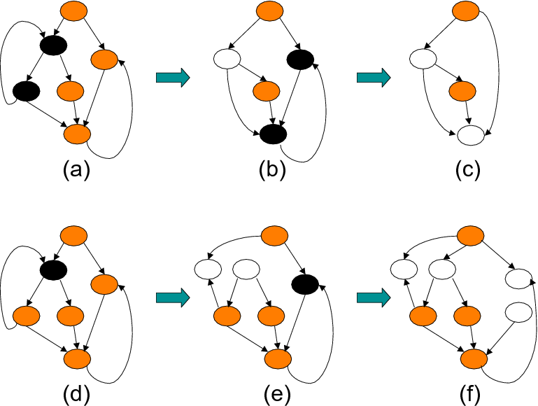
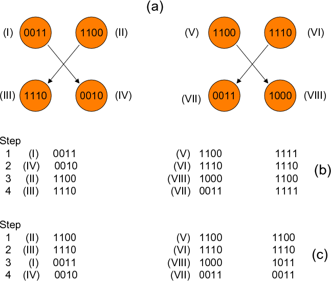
If an LSG has one or more cycles, we need to find a way of eliminating those cycles before the LSG can be scheduled for improving disk reuse. In the rest of this section, we discuss our solution to this issue. It can be observed that there are at least two ways of removing a cycle from a cyclic LSG. First, the nodes that are involved in the cycle can be combined into a single node. This technique is called node merging in this paper, and is illustrated in Figures 7(b) and (c), for the cyclic LSG in Figure 7(a). Note that, when the nodes are merged, the iterations in the combined node can be executed in an order that respect data dependencies. The second technique that can be used for breaking cycles is node splitting (see Figures 7(d) through (f)). While these techniques can be used to convert a non-schedulable LSG to a schedulable one, each has a potential problem we need to be aware of. (clearly, one can also use a combination of node merging and node splitting to remove cycles.) A consequence of node merging is that the corresponding iteration execution may not be very good, as the two successively executed iterations (from the combined node) can access different set of disks. (note that the disk map of the merged node is the bitwise-OR of the disk maps of the involved nodes.) That is, the potential cost of eliminating cycles is a degradation in disk reuse. Node splitting on the other hand has a different problem. It needs to be noted that not all splittings can help us eliminate the cycles in a given LSG. In other words, one needs to be careful in deciding which iterations to place into each of the resulting sub-nodes so that the cyclic dependence at hand can be broken. Determination of these iterations may not be very trivial in practice, but is doable using automated compiler analysis supported by a polyhedral tool. Also, after splitting, the disk maps of the resulting nodes can be determined based on the loop iterations they contain. It is to be observed that node splitting in general also increases the code size as we typically need a separate nest for each node in the LSG.
 |
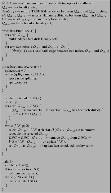
Our preliminary experience with these two techniques showed that in general node splitting is preferable over node merging, mainly because the latter can lead to significant losses in disk reuse, depending on the application code being optimized. Therefore, in our analysis below, we restrict our discussion to node splitting only. However, as mentioned above, code size can be an issue with node splitting, and hence, we keep the number of splittings at minimum. So, the problem now becomes one of determining the minimum number of nodes to split that makes the LSG cycle free. We start by noting that splitting a node, if done successfully, has the same effect as that of removing a node (and the arrows incident on it) from the graph. That is, as far as removing cyclic dependencies is concerned, node splitting and node removal are interchangeable. Fortunately, this latter problem (removing the minimum number of nodes from a graph to make it cycle free) has been studied in the past extensively and is known as the ``feedback vertex set'' problem [8]. Karp was the first one to show that this problem is NP-complete on directed graphs; but it is known today that the undirected version is also NP-complete. Moreover, the problem remains NP-complete for directed graphs with no in-degree or out-degree exceeding 2, and also for planar directed graphs with no in-degree or out-degree exceeding 3. Fortunately, there exist several heuristic algorithms proposed in the literature for the feedback vertex set problem. In this work, we use the heuristic discussed in [7]. Since the details of this heuristic are beyond the scope of this paper, we do not discuss them.
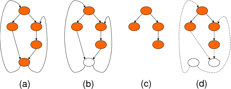
As an example, Figure 8(a) gives a sample LSG. Figure 8(b) highlights the node selected by the heuristic in [7], and Figure 8(c) gives the pruned LSG. Note that splitting the node identified by [7] eliminates both the cycles. Figure 8(d) on the other hand shows the LSG after node splitting, which is cycle free. It is important to note that, while node removal and splitting obviously result in different LSGs, their effects on the schedulability of a given graph are similar; that is, both of them make a given cyclic graph schedulable. In particular, the set of nodes returned by the heuristic in [7] is the set of minimum nodes that need to be considered for splitting (though, as explained below, in some cases we may consider more nodes for potential split). Based on this discussion, Figure 10 gives the algorithm used by our compiler for restructuring a given code for improving disk reuse. This algorithm starts by building the initial LSG for the input code. This LSG can contain cycles, and hence, we next invoke procedure remove_cycles(.) to obtain a cycle free LSG. While this step uses the heuristic approach in [7], it needs to do some other things as well, as explained below.
 |
In the rest of this section, we discuss details of our node splitting strategy. Once a node is identified (using the heuristic in [7]) as a potential candidate for splitting, our approach checks whether it can be split satisfactorily. What is meant by ``satisfactorily'' in this context is that, although in theory we can always a split a node into two or more nodes, the one we are looking for has the properties explained below.
Assume that
![]() is the node to be split. Let
is the node to be split. Let ![]() be the set of nodes from which there are dependencies to node
be the set of nodes from which there are dependencies to node
![]() . That is, for each member,
. That is, for each member,
![]() ,
of
,
of ![]() , there is at least a dependence from
, there is at least a dependence from
![]() to
to
![]() . Assume further that
. Assume further that ![]() is the set of nodes to which we have dependencies from node
is the set of nodes to which we have dependencies from node
![]() . In other words, we have a dependence from
. In other words, we have a dependence from
![]() to each node,
to each node,
![]() , of
, of ![]() . Suppose now that
. Suppose now that
![]() is split into two
sub-nodes:
is split into two
sub-nodes:
![]() and
and
![]() . We
call this split ``satisfactory'' if all of the following three conditions
are satisfied after the split:
. We
call this split ``satisfactory'' if all of the following three conditions
are satisfied after the split:
![]() No dependency goes from any
No dependency goes from any
![]() to
to
![]() . In other words, all the original
in-coming dependencies of
. In other words, all the original
in-coming dependencies of
![]() are directed to
are directed to
![]() .
.
![]() No dependency goes from
No dependency goes from
![]() to any
to any
![]() . In other words, all the original
out-going dependencies of
. In other words, all the original
out-going dependencies of
![]() are directed from
are directed from
![]() .
.
![]() No dependency exists between
No dependency exists between
![]() and
and
![]() .
.
 |
We say that cycle in question is removed (if the removal of
![]() is sufficient to remove the cycle; otherwise, the other
nodes in the cycle, which is detected by the algorithm in
[7], have to be visited), if the three conditions above
are satisfied. It needs to be emphasized that, precisely speaking,
the last condition above is not always necessary.
However, if there exist dependencies between
is sufficient to remove the cycle; otherwise, the other
nodes in the cycle, which is detected by the algorithm in
[7], have to be visited), if the three conditions above
are satisfied. It needs to be emphasized that, precisely speaking,
the last condition above is not always necessary.
However, if there exist dependencies between
![]() and
and
![]() , it is possible that we still have
cycle(s) in the LSG due to
, it is possible that we still have
cycle(s) in the LSG due to
![]() , depending on the
direction of these dependencies. Enforcing the last condition, along
with the others, ensures that the cyclic dependencies are removed
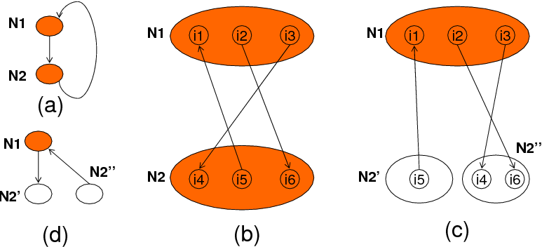
completely. Figure 9 illustrates an example LSG.
Figure 9(a) shows an original LSG in coarse grain and
(b) illustrates the dependencies between the two nodes of this LSG in
fine grain. Assuming that the bottom node has been selected for
removal (ultimately one of possible nodes to be split) by the
heuristic in [7], Figures 9(c) and (d)
show the result of splitting LSG in fine grain and coarse grain,
respectively. As an another example, Figure 8(d)
shows the split version of the LSG in Figure 8(a).
Note that, due to the third condition above, our approach may need to
look at more nodes than ones determined by the heuristic described in
[7]. We also need to mention that, in our
implementation, these three conditions listed above are checked using
the Omega library [26].
, depending on the
direction of these dependencies. Enforcing the last condition, along
with the others, ensures that the cyclic dependencies are removed
completely. Figure 9 illustrates an example LSG.
Figure 9(a) shows an original LSG in coarse grain and
(b) illustrates the dependencies between the two nodes of this LSG in
fine grain. Assuming that the bottom node has been selected for
removal (ultimately one of possible nodes to be split) by the
heuristic in [7], Figures 9(c) and (d)
show the result of splitting LSG in fine grain and coarse grain,
respectively. As an another example, Figure 8(d)
shows the split version of the LSG in Figure 8(a).
Note that, due to the third condition above, our approach may need to
look at more nodes than ones determined by the heuristic described in
[7]. We also need to mention that, in our
implementation, these three conditions listed above are checked using
the Omega library [26].
 |
forIn this code fragment, two disk-resident arrays are accessed (as mentioned earlier, we do not show explicit I/O statements). While one of these is accessed in row wise, the second one is traversed column wise. Consequently, storing both the arrays in the same fashion in file (e.g., as shown in Figure 2) may not be the best option since such a storage will not be able to take advantage of disk reuse for the second array as its data access pattern and file storage pattern would not match. Now, consider the file layout transformation depicted in Figure 11. If this transformation is applied to the second array (=1,
,1
for=1,
![$U[i,j] = f(V[j,i]);$](img70.png)
The important question to address is to select the mapping that
maximizes disk reuse. We start by noting that the search
space is very large for potential file layout transformations, as
there are many ways of transforming a file layout. However, our
experience with disk-intensive scientific applications and our
preliminary experiments suggest that we can restrict the potential
mappings to dimension permutations. What we mean by ``dimension
permutation'' in this context is reindexing the dimensions of the disk
resident array. As an example, restricting ourselves to dimension
re-indexings, a three-dimensional disk-resident array can have 6
different file layouts. Let us use ![]() to represent the disk
mapping function when file layout modification is considered, where
to represent the disk
mapping function when file layout modification is considered, where
![]() is the original disk mapping function discussed earlier in
Section 3 and
is the original disk mapping function discussed earlier in
Section 3 and ![]() is a permutation matrix (that
implements dimension re-indexing). For example, the file layout
mapping shown in Figure 11 can be expressed using the
transformation matrix
is a permutation matrix (that
implements dimension re-indexing). For example, the file layout
mapping shown in Figure 11 can be expressed using the
transformation matrix
It is to be noted, however, that the decision for selection of a
permutation should be made carefully by considering all the statements
that access the array in question. This is because different
statements in the application code can access the same disk-resident
array using entirely different access patterns, and a layout
transformation that does not consider all of them may end up with one
that is not good when considered globally. Our file layout selection
algorithm is a profile based one. In this approach, the
application code is profiled by instrumenting it and attaching a set
of counters to each disk resident array. For an ![]() -dimensional array,
we have
-dimensional array,
we have ![]() counters, each keeping the number of times a particular
file layout is preferred (note that the total number of possible
dimension permutations is
counters, each keeping the number of times a particular
file layout is preferred (note that the total number of possible
dimension permutations is ![]() and one additional counter is used for
representing other file layout preferences such as diagonal layouts,
for which we do not perform any optimization). In this work, we
implement only dimension permutation because other file layouts such
as diagonal layouts or blocked layouts are hardly uniform across all
execution. Therefore, we do not take any actions for such layouts. At
the end of profiling, the layout preference with the largest counter
value is selected as the file layout for that
array. Figure 12 gives the pseudo code for our file
layout selection algorithm. As an example, let us assume that there
are three loop nests (with the same number of iterations) accessing
the same data array stored in a file. Assume further that the
profiling reveals that the first and third loop nests exhibit
column-major access pattern whereas the second loop nest exhibits
row-major access pattern. As the column-major file layout is
preferred more (that is, it will have a higher counter value), we
select the corresponding permutation matrix and convert the file
layout accordingly.
and one additional counter is used for
representing other file layout preferences such as diagonal layouts,
for which we do not perform any optimization). In this work, we
implement only dimension permutation because other file layouts such
as diagonal layouts or blocked layouts are hardly uniform across all
execution. Therefore, we do not take any actions for such layouts. At
the end of profiling, the layout preference with the largest counter
value is selected as the file layout for that
array. Figure 12 gives the pseudo code for our file
layout selection algorithm. As an example, let us assume that there
are three loop nests (with the same number of iterations) accessing
the same data array stored in a file. Assume further that the
profiling reveals that the first and third loop nests exhibit
column-major access pattern whereas the second loop nest exhibits
row-major access pattern. As the column-major file layout is
preferred more (that is, it will have a higher counter value), we
select the corresponding permutation matrix and convert the file
layout accordingly.
 |
![\begin{figure}\centering
\begin{boxedminipage}[t]{0.48\textwidth}
\scriptsize
\b...
... layouts */ \\
\}
\end{tabbing}\end{boxedminipage}\vspace{-0.1in}\end{figure}](img81.png) |
 |
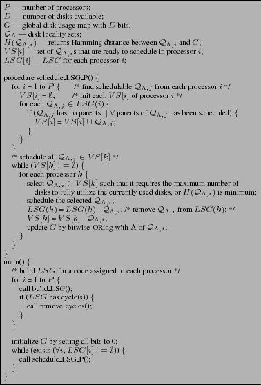
Our scheduling algorithm for an architecture with ![]() processors and
processors and
![]() disks is given in Figure 14. This algorithm takes
the LSGs as input, and determines, for each thread, the schedule of
the nodes considering the global (inter-thread) usage of the disks. It
uses a
disks is given in Figure 14. This algorithm takes
the LSGs as input, and determines, for each thread, the schedule of
the nodes considering the global (inter-thread) usage of the disks. It
uses a ![]() -bit global variable
-bit global variable ![]() to represent the current usage of
the disks. It schedules a node that is ready to be scheduled for each
thread that finishes its current task. At each step, the algorithm
first tries to schedule the node whose disk requirement can be
satisfied with the set of disks currently being used. If multiple
nodes satisfy this criterion, we select the one that requires the
maximum number of disks to make full utilization of the currently used
disks. If such a node does not exist, our algorithm schedules the
node whose tag is the closest (in terms of Hamming Distance) to
to represent the current usage of
the disks. It schedules a node that is ready to be scheduled for each
thread that finishes its current task. At each step, the algorithm
first tries to schedule the node whose disk requirement can be
satisfied with the set of disks currently being used. If multiple
nodes satisfy this criterion, we select the one that requires the
maximum number of disks to make full utilization of the currently used
disks. If such a node does not exist, our algorithm schedules the
node whose tag is the closest (in terms of Hamming Distance) to ![]() ,
the bit pattern that represents the current disk usage (i.e., the disk
usage at that particular point in scheduling). This is to minimize the
number of disks whose (active/idle) states need to be changed. We want
to mention that, since each node may have different execution latency
it is possible that the targeted disk reuse (across threads) may not
always be achieved. However, we can expect the resulting disk reuse
(and buffer performance) to be better than what a random (but legal)
scheduling would achieve.
,
the bit pattern that represents the current disk usage (i.e., the disk
usage at that particular point in scheduling). This is to minimize the
number of disks whose (active/idle) states need to be changed. We want
to mention that, since each node may have different execution latency
it is possible that the targeted disk reuse (across threads) may not
always be achieved. However, we can expect the resulting disk reuse
(and buffer performance) to be better than what a random (but legal)
scheduling would achieve.
 |
Before moving to the discussion of our experimental results, we want to point out the tradeoff between disk reuse and performance. The parallel version of our approach tries to maximize the disk reuse, and this in turn tends to attract the accesses to a small set of disks. Consequently, in theory, this can lead to performance problems, as the effective disk parallelism is reduced. While this negative impact has already been accounted for in our experiments (discussed in the next section), we observed that its magnitude is not very high. However, this magnitude is typically a function of the application access pattern and disk system parameters as well, and further studies are needed to reach better evaluations.
| Parameter | Value |
| CPU | |
| Model | Intel P4 |
| Clock Frequency | 2.6 GHz |
| Memory System | |
| Model | Rambus DRAM |
| Buffer Capacity | 1 GB |
| Disk System | |
| Number of I/O Nodes | 8 |
| Data Striping | Uses all 8 I/O nodes |
| Stripe Size | 64 KB |
| Interface | ATA |
| Storage Capacity/Disk | 40 GB |
| RPM | 10,000 |
| Interconnect | |
| Model | Ethernet |
| Bandwidth | 100 Mbps |
We performed our experiments using a platform which includes MPI-IO [33] on top of the PVFS parallel file system [27]. PVFS is a parallel file system that stripes file data across multiple disks in different nodes in a cluster. It accommodates multiple user interfaces which include MPI-IO, traditional Linux interface, and the native PVFS library interface. In all our experiments, we used the MPI-IO interface. Table 1 gives the values of our major experiment parameters. We want to emphasize however that later we present results from our sensitivity analysis where we change the default values of some of the important parameters.
For each benchmark in our experimental suite, we performed experiments with different versions:
![]() Base Scheme: This represents the original code without any
data locality optimization.
Base Scheme: This represents the original code without any
data locality optimization.
![]() Conventional Locality Optimization (CLO): This represents
a conventional data locality optimization technique that employs loop
restructuring. It is not designed for I/O, and does not take disk
layout into account. The specific data reuse optimizations used
include loop interchange, loop fusion, iteration tiling and
unrolling. This version in a sense represents the state-of-the-art as
far as data locality optimization is concerned.
Conventional Locality Optimization (CLO): This represents
a conventional data locality optimization technique that employs loop
restructuring. It is not designed for I/O, and does not take disk
layout into account. The specific data reuse optimizations used
include loop interchange, loop fusion, iteration tiling and
unrolling. This version in a sense represents the state-of-the-art as
far as data locality optimization is concerned.
![]() Disk Reuse Optimization - Loop Based (DRO-L): This is our
approach applied at a loop nest level; i.e., each loop nest is
optimized in isolation.
Disk Reuse Optimization - Loop Based (DRO-L): This is our
approach applied at a loop nest level; i.e., each loop nest is
optimized in isolation.
![]() Disk Reuse Optimization - Whole Program Based (DRO-WP):
This is our approach applied at a whole program level.
Disk Reuse Optimization - Whole Program Based (DRO-WP):
This is our approach applied at a whole program level.
All the versions use the MPI-IO interface [33] of PVFS [27] for performing disk I/O. Note that both DRO-L and DRO-WP are the different versions of our approach, and CLO represents the state-of-the-art as far as optimizing data locality is concerned. The reason that we make experiments with the DRO-L and DRO-WP versions separately is to see how much additional benefits one can obtain by going beyond the loop nest level in optimizing for I/O. In addition to these versions, we also implemented and conducted experiments with the file layout optimization scheme discussed in Section 4 and with the parallel version of our approach explained in Section 5.
| Application | Brief | Data Set | Disk I/O | Total |
| Name | Description | Size (GB) | Time (sec) | Time (sec) |
| sar | Synthetic Aperture Radar Kernel | 21.1 | 64.6 | 101.4 |
| hf | Hartree-Fock Method | 53.6 | 98.3 | 173.6 |
| apsi | Pollutant Distribution Modeling | 49.9 | 101.2 | 238.7 |
| wupwise | Physics/Quantum Chromo-dynamics | 27.9 | 270.3 | 404.7 |
| e_elem | Finite Element Electromagnetic Modeling | 66.2 | 99.2 | 191.9 |
| astro | Analysis of Astronomical Data | 58.3 | 171.6 | 276.4 |
| contour | Contour Displaying | 58.7 | 198.6 | 338.4 |
The unit of buffer (cache) management in our implementation is a data block, and its size is the same as that of a stripe. The set of applications used in this study is given in Table 2. These applications are collected from different sources and their common characteristic is that they are disk-intensive. apsi and wupwise are similar to their Spec2000 counterparts [14], except that they operate on disk-resident data. The second column briefly explains each benchmark, and the third column gives the total (disk resident) data set size processed by each application. The fourth and fifth columns give the disk I/O times and total execution times, respectively, under the base scheme explained above. Note that both the base version and the CLO version are already optimized for buffer usage. In addition, the CLO version is optimized for data locality using conventional techniques, as explained above. Therefore, the performance improvements brought by our approaches (DRO-L and DRO-WP) over these schemes (base and CLO) are due to the code re-ordering we apply. We also see from Table 2 that the contribution of disk I/O times to overall execution times varies between 42.4% and 63.7%, averaging on 57.4%. Therefore, reducing disk I/O times can be very useful in practice. In the remainder of this section, we present and discuss the performance improvements brought by our approach. The disks I/O time savings and overall execution time savings presented below are with respect to the fourth and fifth columns of Table 2, respectively.
|
|
|
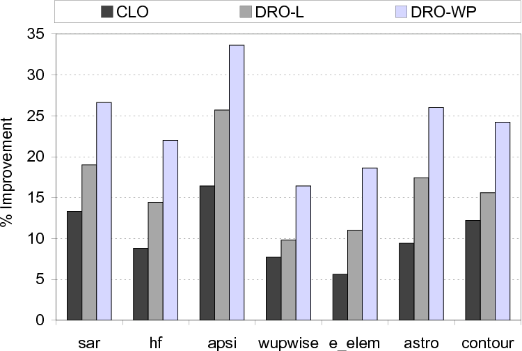
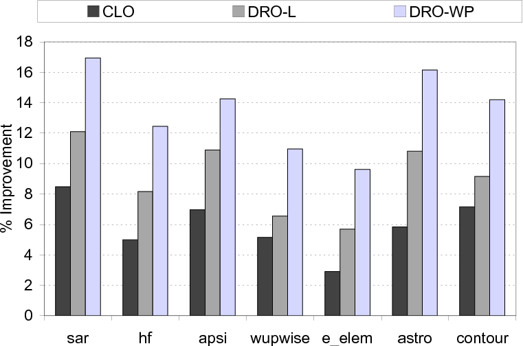
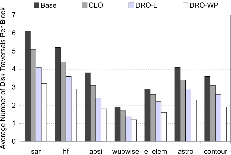
We start by presenting the percentage improvements in disk I/O times brought by the three optimized versions explained above. The results shown in Figure 15 indicate that the average improvements brought by CLO, DRO-L and DRO-WP over the base scheme are 10.4%, 16.1% and 23.9%, respectively. Overall, we see that, while DRO-L performs better than CLO, by 6.3% on average, the best savings are obtained - for all benchmarks tested - with the DRO-WP version, on average, 15.0% and 9.3% over CLO and DRO-L, respectively, meaning that going beyond a single loop nest is important in maximizing the buffer performance. While these improvements in disk I/O times are important, we also need to look at the savings in overall execution times, which include the computation times as well. These results are presented in Figure 16 and show that the average improvements with the CLO, DRO-L and DRO-WP versions are 5.9%, 9.0% and 13.5%, respectively. To better explain how our approach achieves much more performance improvements over conventional data reuse optimization, we present in Figure 17 the average number of times a given data block is visited under the different schemes (that is, how many times a given data block (on average) is brought from disks to cache). We observe that this number is much lower with the DRO-WP version, explaining the additional performance benefits it brings. In fact, on average, the number of disk traversals per block is 3.9 and 2.1 with the base version and DRO-WP, respectively.
|
|
|
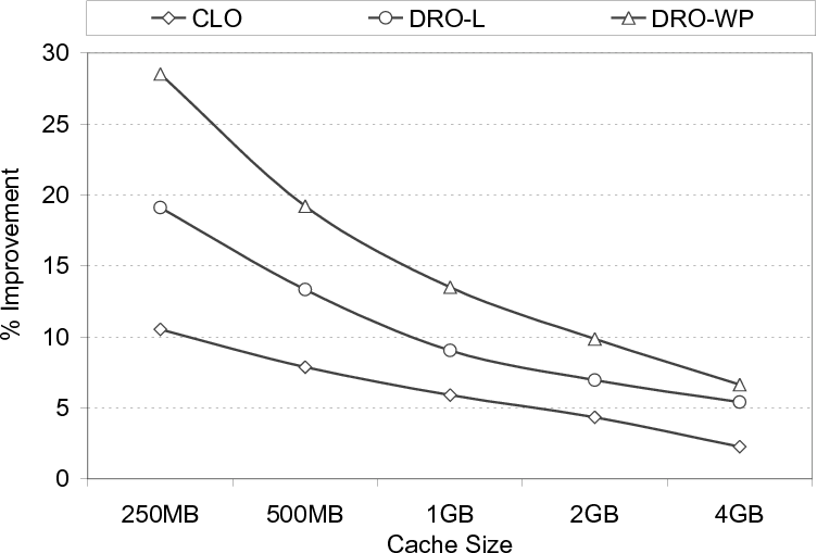
Sensitivity Analysis.
In this section, we study the sensitivity of our performance savings
to several parameters. A critical parameter of interest is the buffer
(cache) size. Recall that the default buffer size used in our
experimental evaluation so far was 1GB. The graph in Figure 18
gives the results using different buffer sizes. Each point in this
graph represents the average value (performance improvement in overall
execution time), for a given version, when all seven benchmarks are
considered. As expected, the performance gains brought by our approach
get reduced when increasing the buffer size. However, even with the
largest buffer size we used, the average improvement we have (with the
DRO-WP version) is about 6.7%, underlining the importance of disk
reuse optimization for better performance. Considering the fact that
data set sizes of disk-intensive applications keep continuously
increasing, one can expect the disk reuse based approach to be more
effective in the future. To elaborate on this issue further, we also
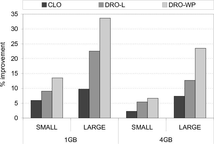
performed experiments with larger data sets. Recall that the third column
of Table 2 gives the data set sizes used in our
experiments so far. Figure 19 gives the average performance
improvements, for 1GB and 4GB buffer sizes and two sets of inputs.
SMALL refers to the default dataset sizes given in Table 2,
and LARGE refers to larger datasets, which are 38.2GB, 66.3GB, 82.1GB,
38.0GB, 88.1GB, 73.7GB, and 81.8GB for sar, hf, apsi, wupwise, e_elem,
astro and contour, respectively. We see that our approach performs better
with larger data set sizes. This is because a larger data set puts more
pressure on the buffer, which makes effective utilization of buffer even
more critical.
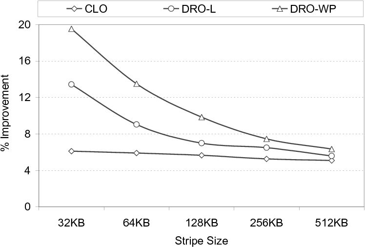
The next parameter we study is the stripe size, which can also be changed using a PVFS call when creating the file. The performance improvement results with different stripe sizes are presented in Figure 20. Our observation is that the DRO-WP version generates the best results with all stripe sizes tested. We also see that the performance savings are higher with smaller stripe sizes. This can be explained as follows. The disk reuse is not very good in the original codes (the base scheme) with smaller stripe sizes, and since the savings shown are normalized with respect to the original codes, we observe large savings.
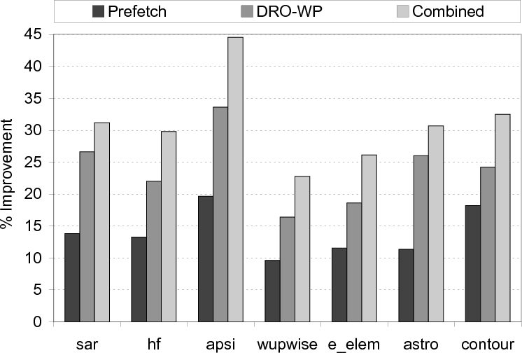
Comparison with I/O Prefetching.
We next compare our approach to prefetching. The specific prefetch
implementation we use is inspired by TIP [24], a hint-based
I/O prefetching scheme. The graph in Figure 21
presents, for each benchmark, three results: prefetching alone, DRO-WP
alone, and the two technique combined. We see from these results that
the best performance improvements are achieved using both prefetching
and code restructuring. This is because these two optimization
techniques are in a sense orthogonal to each other. Specifically,
while core restructuring tries to reduce I/O latencies by
improving buffer performance, prefetching tries to hide I/O
latencies. While it is also possible to integrate these two
optimizations better (rather than applying one after another), we
postpone exploring this option to a future study.
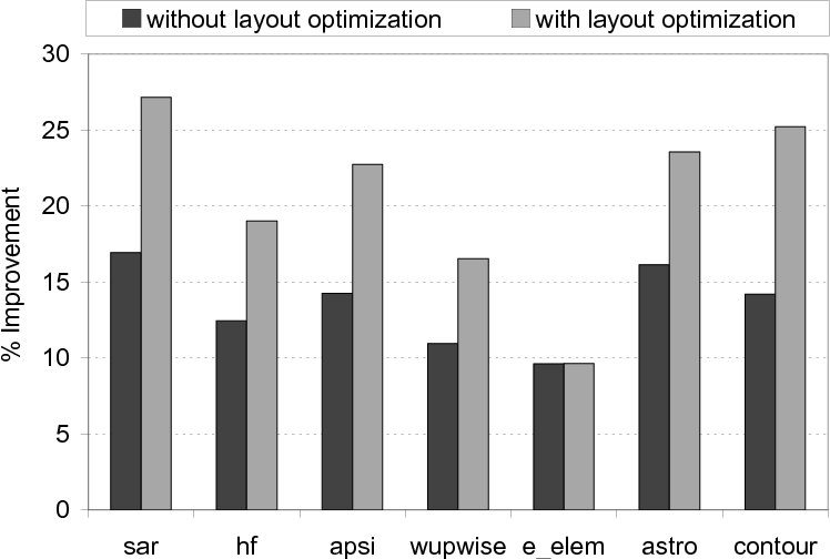
Impact of File Layout Optimization.
Recall from Section 4 that file layout optimization
(which impacts the layout of data on the disks as well) can
help our approach improve disk reuse further. To quantify this, we
performed another set of experiments, whose results are presented in
Figure 22 when the whole program is optimized. We see
that, except for one benchmark, layout optimization improves the
effectiveness of our code restructuring approach. The average
additional improvement it brings is about 7%. We observe that
the file layout optimization could not find much opportunity for
improvement in benchmark e_elem as the default file layouts of the
disk resident arrays in this benchmark perform very well.
|
|
|
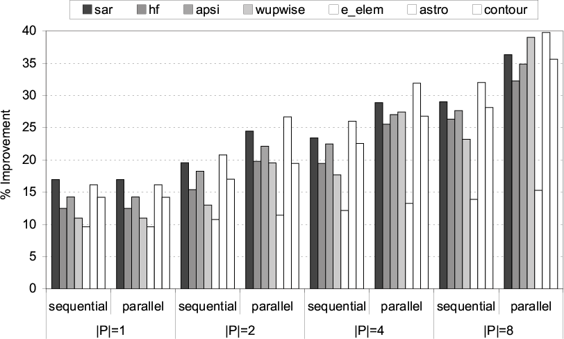
Evaluation of Parallel Execution.
Figure 23 presents the results collected from an
evaluation of the parallel version of our approach discussed in
Section 5. For these experiments, the number of CPUs
that are used to execute an application is varied between 1 and 8. For
each processor size, we present the results with our baseline
implementation (where disk reuse is optimized from each CPU's
perspective individually) as well as with those obtained when the
approach in Section 5 is enabled. We see from these
results that considering all parallel threads together is important in
maximizing overall disk reuse, especially with the large number of
CPUs. For example, when 8 CPUs are used for executing an application,
the average performance improvements with individual reuse
optimization (sequential version) and collective reuse optimization
(parallel version) are 25.7% and 33.3%, respectively.
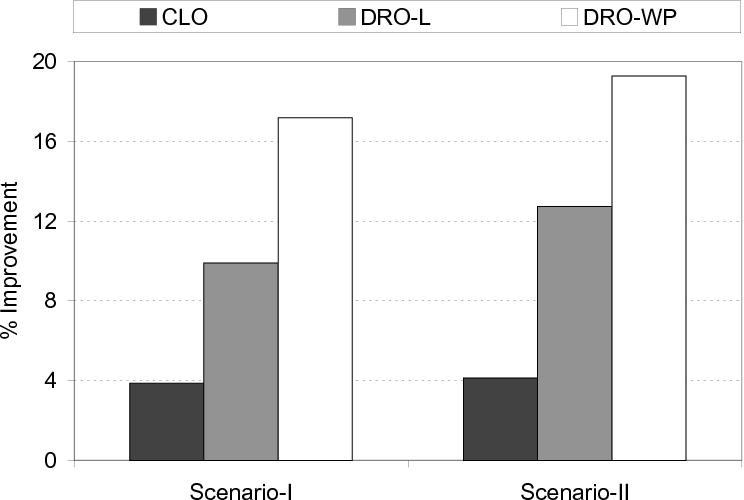
Evaluation of Multiple Application Execution.
Since a disk system can be used by multiple applications at the same
time, it is also important to quantify the benefits brought by our
approach under such an execution scenario. Figure 24
presents the results from two sets of experiments. In the first set,
called Scenario-I, 7 CPUs are used and each CPU executes one of our
seven applications. In the second set, called Scenario-II, 8 CPUs are
used and four of our applications (sar, hf, apsi and astro) are
parallelized, each using two CPUs. In both set of experiments, a CPU
executes only a single thread. Also, in Scenario-I the sequential
version of our approach is used (for each application), and in
Scenario-II the parallel version explained in
Section 5 is used. The results given in
Figure 24 indicate that the DRO-WP version generates the
best results for both the scenarios tested.
There has been significant past work on optimizing file and buffer cache management in storage systems [3,9,10,16,28,35]. To better exploit multi-level caches, which are common in modern storage systems, several multi-level buffer cache management policies have been proposed [6,37,35]. [37] introduced a DEMOTE operation that allows one to keep cache blocks in an exclusive manner, i.e., a cache block is not duplicated across cache hierarchy. Chen et al [6], on the other hand, utilize the eviction information of higher level cache in deciding which cache blocks need to be replaced in a lower level of the cache hierarchy. More recently, [38] proposed a replacement policy for multi-level cache, called Karma. Karma uses application hints in maintaining cache blocks exclusively. Most high-end parallel and cluster systems provide some sort of parallel I/O operations to meet the I/O requirements (i.e., low latency and high bandwidth) of scientific applications. This is typically accomplished by employing a set of I/O nodes, each of which is equipped with multiple disks, dividing a file into a number of small file stripes, and distributing those stripes across available I/O nodes. This notion of file-level striping is adapted in many commercial or research parallel file systems, such as IBM GPFS [28], Intel PFS [11], PPFS [15], Galley [22], and PVFS2 [27]. It should be mentioned that these parallel file systems provide huge I/O performance improvements when they receive large and contiguous I/O requests. However, many scientific applications that exhibit small and non-contiguous I/O access patterns may suffer from performance degradation. To deal with this problem, several approaches have been proposed in the context of different parallel file system libraries and APIs such as Panda [5], PASSION [31], and MPI-IO [32,33,34]. Among various techniques used to achieve this goal, collective I/O is commonly recognized as an efficient way of reducing I/O latency. The concept of collective I/O can be implemented in different places of parallel I/O systems; namely, client side [34], disk side [19], or server side [29]. The majority of the existing collective I/O implementations employ two-phase I/O [34]. In two-phase I/O, disk accesses are reorganized in client side (compute node) before sending them over the I/O nodes. Disk-directed I/O [19], on the other hand, performs collective I/O operations on disk side, where I/O requests are optimized such that they conform to the storage layouts. In Panda [29], I/O server nodes, rather than disk or client nodes, generate I/O requests that conform to the layouts of disk-resident array data.
Our approach is different from prior compiler-based I/O optimization techniques in that it optimizes entire program rather than individual, parallel loop nests. It is also different from previous studies that considered buffer caching and prefetching because we improve I/O performance by increasing disk reuse. Lastly, our approach emphasizes the role of file layout optimization and parallel execution when applying optimization techniques to achieve better disk reuse (and better cache performance).
Acknowledgments
This work is supported in part by the NSF grants #0406340, #0444158,
and #0621402. We would like to thank our anonymous reviewers
for their helpful comments.
This document was generated using the LaTeX2HTML translator Version 2002-2-1 (1.71)
Copyright © 1993, 1994, 1995, 1996,
Nikos Drakos,
Computer Based Learning Unit, University of Leeds.
Copyright © 1997, 1998, 1999,
Ross Moore,
Mathematics Department, Macquarie University, Sydney.
The command line arguments were:
latex2html -split 0 -show_section_numbers -local_icons -no_navigation son_html.tex
The translation was initiated by Seung Son on 2008-01-08