| ||||||||||||||||||||||||||||||||||||||||||||||||||||
|
OSDI '04 Paper
[OSDI '04 Technical Program]
Correlating instrumentation data to system states:
|
 |
To explore TANs as a basis for self-managing systems, we analyzed data from 124 metrics gathered from a three-tier e-commerce site under synthetic load. The induced TAN models select combinations of metrics and threshold values that correlate with high-level performance states--compliance with Service Level Objectives (SLO) for average response time--under a variety of conditions. The experiments support the following conclusions:
Of the known statistical learning techniques, the TAN structure and algorithms are among the most promising for deployment in real systems. They are based on sound and well-developed theory, they are computationally efficient and robust, they require no expertise to use, and they are readily available in open-source implementations [24,34,5]. While other approaches may prove to yield comparable accuracy and/or efficiency, Bayesian networks and TANs in particular have important practical advantages: they are interpretable and they can incorporate expert knowledge and constraints. Although our primary emphasis is on diagnosing performance problems after they have occurred, we illustrate the versatility of TANs by using them to forecast problems. We emphasize that our methods discover correlations rather than causal connections, and the results do not yet show that a robust ``closed loop'' diagnosis is practical at this stage. Even so, the technique can sift through a large amount of instrumentation data rapidly and focus the attention of a human analyst on the small set of metrics most relevant to the conditions of interest.
This paper is organized as follows: Section 2 defines the problem and gives an overview of our approach. Section 3 gives more detail on TANs and the algorithms to induce them, and outlines the rationale for selecting this technique for computer systems diagnosis and control. Section 4 describes the experimental methodology and Section 5 presents results. Section 6 presents additional results from a second testbed to confirm the diagnostic power of TANs. Section 7 discusses related work, and Section 8 concludes.
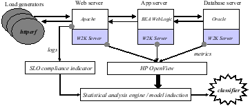
Figure 1 depicts the experimental environment. The system under test is a three-tier Web service: the Web server (Apache), application middleware server (BEA WebLogic), and database server (Oracle) run on three different servers instrumented with HP OpenView to collect a set of system metrics. A load generator (httperf [28]) offers load to the service over a sequence of execution intervals. An SLO indicator processes the Apache logs to determine SLO compliance over each interval, based on the average server response time for requests in the interval.
This paper focuses on the problem of constructing an analysis engine to process the metrics and indicator values. The goal of the analysis is to induce a classifier, a function that predicts whether the system is or will be in compliance over some interval, based on the values of the metrics collected. If the classifier is interpretable, then it may also be useful for diagnostic forensics or control. One advantage of our approach is that it identifies sets of metrics and threshold values that correlate with SLO violations. Since specific metrics are associated with specific components, resources, processes, and events within the system, the classifier indirectly identifies the system elements that are most likely to be involved with the failure or violation. Even so, the analysis process is general because it uses no a priori knowledge of the system's structure or function.
In this study we limit our attention to system-level metrics gathered from a standard operating system (Windows 2000 Server) on each of the servers. Of course, the analysis engine may be more effective if it considers application-level metrics; on the other hand, analysis and control using system-level metrics can generalize to any application. Table 1 lists some specific system-level metrics that are often correlated with SLO violations.
This problem is a pattern classification problem in supervised
learning. Let ![]() denote the state of the SLO at time
denote the state of the SLO at time ![]() . In
this case,
. In
this case, ![]() can take one of two states from the set
can take one of two states from the set
![]() : let
: let ![]() or
or ![]() denote these states.
Let
denote these states.
Let ![]() denote a vector of values for
denote a vector of values for ![]() collected metrics
collected metrics
![]() at time
at time ![]() (we will omit the subindex
(we will omit the subindex ![]() when the
context is clear). The pattern classification problem is to induce
or learn a classifier function
when the
context is clear). The pattern classification problem is to induce
or learn a classifier function ![]() mapping the universe of
possible values for
mapping the universe of
possible values for ![]() to the range of system states
to the range of system states
![]() [16,7].
[16,7].
The input to this analysis is a training data set. In this case,
the training set is a log of
observations of the form
![]() from the system in operation. The learning is
supervised in that the SLO compliance indicator identifies the value
of
from the system in operation. The learning is
supervised in that the SLO compliance indicator identifies the value
of ![]() corresponding to each observed
corresponding to each observed ![]() in the training
set, providing preclassified instances for the analysis to learn
from.
in the training
set, providing preclassified instances for the analysis to learn
from.
We emphasize four premises that are implicit in this problem statement. First, it is not necessary to predict system behavior, but only to identify system states that correlate with particular failure events (e.g., SLO violations). Second, the events of interest are defined and identified externally by some failure detector. For example, in this case it is not necessary to predict system performance, but only to classify system states that comply with an SLO as specified by an external indicator. Third, there are patterns among the collected metrics that correlate with SLO compliance; in this case, the metrics must be well-chosen to capture system states relating to the behavior of interest. Finally, the analysis must observe a statistically significant sample of event instances in the training set to correlate states with the observed metrics. Our approach is based on classification rather than anomaly detection: it trains the models with observations of SLO violations as well as normal behavior. The resulting models are useful to predict and diagnose performance problems.
The key measure of success is the accuracy of the
resulting classifier ![]() . A common metric is the classification
accuracy, which in this case
is defined as the probability that
. A common metric is the classification
accuracy, which in this case
is defined as the probability that ![]() correctly identifies the SLO state
correctly identifies the SLO state ![]() associated with any
associated with any
![]() . This measure can be misleading when violations
are uncommon: for example, if
. This measure can be misleading when violations
are uncommon: for example, if ![]() of the intervals violate
the SLO, a trivial classifier that always
guesses compliance yields a classification
accuracy of
of the intervals violate
the SLO, a trivial classifier that always
guesses compliance yields a classification
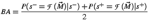
accuracy of ![]() . Instead, our figure of merit is balanced
accuracy (BA), which averages the probability of correctly
identifying compliance with the probability of detecting a violation.
Formally:
. Instead, our figure of merit is balanced
accuracy (BA), which averages the probability of correctly
identifying compliance with the probability of detecting a violation.
Formally:
To achieve the maximal BA of ![]() ,
, ![]() must perfectly
classify both SLO violation and SLO compliance. The trivial
classifier in the example above has a BA of only
must perfectly
classify both SLO violation and SLO compliance. The trivial
classifier in the example above has a BA of only ![]() . In some
cases we can gain more insight into the behavior of a classifier by
considering the false positive rate and false negative rate
separately.
. In some
cases we can gain more insight into the behavior of a classifier by
considering the false positive rate and false negative rate
separately.
There are many techniques for pattern classification in the
literature (e.g., [7,30]). Our
approach first induces a model of the relationship between
![]() and
and ![]() , and then uses the model to decide whether any
given set of metric values
, and then uses the model to decide whether any
given set of metric values ![]() is more likely to correlate with
an SLO violation or compliance. In our case, the model represents
the conditional distribution
is more likely to correlate with
an SLO violation or compliance. In our case, the model represents
the conditional distribution ![]() --the distribution of
probabilities for the system state given the observed values of the
metrics. The classifier then uses this distribution to evaluate
whether
--the distribution of
probabilities for the system state given the observed values of the
metrics. The classifier then uses this distribution to evaluate
whether
![]() .
.
Thus, we transform the problem of pattern classification to one of statistical fitting of a probabilistic model. The key to this approach is to devise a way to represent the probability distribution that is compact, accurate, and efficient to process. Our approach represents the distribution as a form of Bayesian network (Section 3).
An important strength of this
approach is that one can interrogate
the model to identify specific metrics that affect the classifier's
choice for any given ![]() . This interpretability
property
makes Bayesian networks attractive for diagnosis and control,
relative to competing alternatives such as neural networks and
support vector machines [13].
One other alternative, decision
trees [30], can be interpreted as a set of if-then
rules on the metrics and their values.
Bayesian networks have an additional advantage of modifiability:
they can incorporate expert knowledge or constraints
into the model efficiently. For example, a user can specify a subset
of metrics or correlations to include in the model, as discussed
below. Section 3.3 outlines the formal basis
for these properties.
. This interpretability
property
makes Bayesian networks attractive for diagnosis and control,
relative to competing alternatives such as neural networks and
support vector machines [13].
One other alternative, decision
trees [30], can be interpreted as a set of if-then
rules on the metrics and their values.
Bayesian networks have an additional advantage of modifiability:
they can incorporate expert knowledge or constraints
into the model efficiently. For example, a user can specify a subset
of metrics or correlations to include in the model, as discussed
below. Section 3.3 outlines the formal basis
for these properties.
The key challenge for our approach is that it is intractable to induce the optimal Bayesian network classifier. Heuristics may guide the search for a good classifier, but there is also a risk that a generalized Bayesian network may overfit data from the finite and possibly noisy training set, compromising accuracy. Instead, we restrict the form of the Bayesian network to a TAN (Section 3) and select the optimal TAN classifier over a heuristically selected subset of the metrics. This approach is based on the premise (which we have validated empirically in our domain) that a relatively small subset of metrics and threshold values is sufficient to approximate the distribution accurately in a TAN encoding relatively simple dependence relationships among the metrics. Although the effectiveness of TANs is sensitive to the domain, TANs have been shown to outperform generalized Bayesian networks and other alternatives in both cost and accuracy for classification tasks in a variety of contexts [18]. This paper evaluates the efficiency and accuracy of the TAN algorithm in the context of SLO maintenance for a three-tier Web service, and investigates the nature of the induced models.
Before explaining the approach in detail, we first consider its potential impact in practice. We are interested in using classifiers to diagnose a failure or violation condition, and ultimately to repair it.
The technique can be used for diagnostic forensics as follows. Suppose a developer or operator wishes to gain insight into a system's behavior during a specific execution period for which metrics were collected. Running the algorithm yields a classifier for any event--such as a failure condition or SLO threshold violation--that occurs a sufficient number of times to induce a model (see Section 3). In the general case, the event may be defined by any user-specified predicate (indicator function) over the metrics. The resulting model gives a list of metrics and ranges of values that correlate with the event, selected from the metrics that do not appear in the definition of the predicate.
The user may also ``seed'' the models by preselecting a set of metrics that must appear in the models, and the value ranges for those metrics. This causes the algorithm to determine the degree to which those metrics and value ranges correlate with the event, and to identify additional metrics that are maximally correlated subject to the condition that the values of the specified metrics are within their specified ranges. For example, a user can ask a question of the form: ``what percentage of SLO violations occur during intervals when the network traffic between the application server and the database server is high, and what other metrics and values are most predictive of SLO violations during those intervals''?
The models also have potential to be useful for online forecasting of failures or SLO violations. For example, Section 5 shows that it is possible to induce models that predict SLO violations in the near future, when the characteristics of the workload and system are stable. An automated controller may invoke such a classifier directly to identify impending violations and respond to them, e.g., by shedding load or adding resources.
Because the models are cheap to induce, the system may refresh them periodically to track changes in the workload characteristics and their interaction with the system structure. In more dynamic cases, it is possible to maintain multiple models in parallel and select the best model for any given period. The selection criteria may be based on recent accuracy scores, known cyclic behavior, or other recognizable attributes.
 |
This section gives more detail on the TAN representation and algorithm, and discusses the advantages of this approach relative to its alternatives.
As stated in the previous section, we use TANs to obtain a compact,
efficient representation of the model underlying the classifier. The
model approximates a probability distribution ![]() , which
gives the probability that the system is in any given state
, which
gives the probability that the system is in any given state ![]() for
any given vector of observed metrics
for
any given vector of observed metrics ![]() .
Inducing a model of this form reduces to
fitting the distribution
.
Inducing a model of this form reduces to
fitting the distribution ![]() --the probability of
observing a given vector
--the probability of
observing a given vector ![]() of metric values when the system
is in a given state
of metric values when the system
is in a given state ![]() .
Multidimensional
problems of this form are subject to challenges of robustness and
overfitting, and require a large number
of data samples [16,21].
We can simplify the problem
by making some assumptions about the structure
of the distribution
.
Multidimensional
problems of this form are subject to challenges of robustness and
overfitting, and require a large number
of data samples [16,21].
We can simplify the problem
by making some assumptions about the structure
of the distribution ![]() .
TANs comprise a subclass of
Bayesian networks [29], which offer a well-developed
mathematical language to represent structure in probability
distributions.
.
TANs comprise a subclass of
Bayesian networks [29], which offer a well-developed
mathematical language to represent structure in probability
distributions.
A Bayesian network is an annotated directed acyclic graph encoding a
joint probability distribution. The vertices in the graph represent
the random variables of interest in the domain to be modeled, and the
edges represent direct influences of one variable on another. In
our case, each system-level metric ![]() is a random variable
represented in the graph. Each vertex in the network encodes
a probability distribution on the values that the random variable can
take, given the state of its predecessors. This representation
encodes a set of (probabilistic) independence statements of the form:
each random variable is independent of its non-descendants, given
that the state of its parents is known.
There is a set of well-understood
algorithms and methods to induce Bayesian network
models statistically from
data [22], and these are
available in open-source software [24,34,5].
is a random variable
represented in the graph. Each vertex in the network encodes
a probability distribution on the values that the random variable can
take, given the state of its predecessors. This representation
encodes a set of (probabilistic) independence statements of the form:
each random variable is independent of its non-descendants, given
that the state of its parents is known.
There is a set of well-understood
algorithms and methods to induce Bayesian network
models statistically from
data [22], and these are
available in open-source software [24,34,5].
In a naive Bayesian network, the state variable ![]() is the only
parent of all other vertices. Thus a naive Bayesian network assumes
that all the metrics are fully independent given
is the only
parent of all other vertices. Thus a naive Bayesian network assumes
that all the metrics are fully independent given ![]() . A
tree-augmented naive Bayesian network (TAN) extends this structure
to consider
relationships among the metrics themselves, with the constraint
that each metric
. A
tree-augmented naive Bayesian network (TAN) extends this structure
to consider
relationships among the metrics themselves, with the constraint
that each metric ![]() has at most one parent
has at most one parent ![]() in the network other
than
in the network other
than ![]() . Thus a TAN imposes a tree-structured dependence graph on a
naive Bayesian network; this structure is a Markov tree.
The TAN for a set of observations and metrics is defined as the
Markov tree that is optimal in the sense that it has the
highest probability of having generated the observed data [18].
. Thus a TAN imposes a tree-structured dependence graph on a
naive Bayesian network; this structure is a Markov tree.
The TAN for a set of observations and metrics is defined as the
Markov tree that is optimal in the sense that it has the
highest probability of having generated the observed data [18].
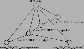
Figure 2 illustrates a TAN obtained for
one of our experiments (see the
STEP workload in Section 4.1.2). This model
has a balanced accuracy (BA) score of ![]() for the system,
workload, and SLO in that experiment. The metrics selected are the
variance of the CPU user time at the application server, network
traffic (packets and bytes) from that server to the
database tier, and the swap space and disk activity at the
database. The tree structure captures the
following assertions: (1) given the network traffic
between the tiers, the
CPU activity in the application server is irrelevant to the swap space
and disk activity at the database tier; (2) the network traffic
is correlated with CPU
activity, i.e., common increases in the values of those
metrics are not anomalous.
for the system,
workload, and SLO in that experiment. The metrics selected are the
variance of the CPU user time at the application server, network
traffic (packets and bytes) from that server to the
database tier, and the swap space and disk activity at the
database. The tree structure captures the
following assertions: (1) given the network traffic
between the tiers, the
CPU activity in the application server is irrelevant to the swap space
and disk activity at the database tier; (2) the network traffic
is correlated with CPU
activity, i.e., common increases in the values of those
metrics are not anomalous.
Our TAN models approximate the probability distribution of values for each metric (given the value of its predecessor) as a conditional Gaussian distribution. This method is efficient and avoids problems of discretization. The experimental results show that it has acceptable accuracy and is effective in capturing the abnormal metric values associated with each performance state. Other representations may be used with the TAN technique.
Given a basic understanding of the classification approach and the
models, we now outline the methods and algorithms
used to select the TAN model for the classifier (derived from [18]).
The goal is to select a subset ![]() of
of ![]() whose TAN yields the most accurate classifier, i.e.,
whose TAN yields the most accurate classifier, i.e., ![]() includes the metrics from
includes the metrics from ![]() that correlate most
strongly with SLO violations observed in the data.
Let
that correlate most
strongly with SLO violations observed in the data.
Let ![]() be the size of the subset
be the size of the subset ![]() .
The problem of selecting the best
.
The problem of selecting the best ![]() metrics for
metrics for ![]() is known as
feature selection. Most solutions use some form of heuristic
search given the combinatorial explosion of the search space in the
number of metrics in
is known as
feature selection. Most solutions use some form of heuristic
search given the combinatorial explosion of the search space in the
number of metrics in ![]() . We use a greedy strategy: at each
step select the metric that is not already in the vector
. We use a greedy strategy: at each
step select the metric that is not already in the vector
![]() , and that yields maximum improvement in accuracy (BA)
of the resulting TAN over the sample data. To
do this, the algorithm computes the optimal Markov tree for each candidate
metric, then selects the metric whose tree
yields the highest BA score
against the observed data.
The cost is
, and that yields maximum improvement in accuracy (BA)
of the resulting TAN over the sample data. To
do this, the algorithm computes the optimal Markov tree for each candidate
metric, then selects the metric whose tree
yields the highest BA score
against the observed data.
The cost is ![]() times the cost to
induce and evaluate the Markov tree, where
times the cost to
induce and evaluate the Markov tree, where ![]() is the number
of metrics. The algorithm to find the
optimal Markov tree computes a minimum spanning tree
over the metrics in
is the number
of metrics. The algorithm to find the
optimal Markov tree computes a minimum spanning tree
over the metrics in ![]() .
.
From Eq. 1 it is clear that to compute a candidate's BA score we must estimate the probability of false positives and false negatives for the resulting model. The algorithm must approximate the real BA score from a finite set of samples. To ensure the robustness of this score against variability on the unobserved cases in the data, the following procedure called ten-fold cross validation is used [21]. Randomly divide the data into two sets, a training set and a testing set. Then, induce the model with the training set, and compute its score with the testing set. Compute the final score as the average score over ten trials. This reduces any biases or overfitting effects resulting from a finite data set.
Given a data set with ![]() samples of the
samples of the ![]() metrics, the overall
algorithm is dominated by
metrics, the overall
algorithm is dominated by ![]() for small
for small ![]() , when all
, when all ![]() samples are used to induce and test the candidates.
Most of our experiments train models for
samples are used to induce and test the candidates.
Most of our experiments train models for ![]() SLO definitions on
stored instrumentation datasets with
SLO definitions on
stored instrumentation datasets with ![]() and
and ![]() . Our
Matlab implementation processes each dataset in about ten minutes on a
1.8 GHz Pentium 4 (
. Our
Matlab implementation processes each dataset in about ten minutes on a
1.8 GHz Pentium 4 (![]() seconds per SLO). Each run induces about
40,000 candidate models, for a rough average of 15 ms per model. Once
the model is selected, evaluating it to classify a new interval sample
takes 1-10 ms. These operations are cheap enough to train models
online as needed and even to maintain and evaluate multiple models in
parallel.
seconds per SLO). Each run induces about
40,000 candidate models, for a rough average of 15 ms per model. Once
the model is selected, evaluating it to classify a new interval sample
takes 1-10 ms. These operations are cheap enough to train models
online as needed and even to maintain and evaluate multiple models in
parallel.
In addition to their efficiency in representation and inference, TANs (and Bayesian networks in general) present two key practical advantages: interpretability and modifiability. These properties are especially important in the context of diagnosis and control.
The influence of each metric on the violation of an SLO can be
quantified in a sound probabilistic model.
Mathematically, we arrive at the following functional form for the
classifier as a sum of terms, each involving the probability that the
value of some metric ![]() occurs in each state given the value of its
predecessor
occurs in each state given the value of its
predecessor ![]() :
:
This structure gives insight into the causes of the violation or even how to repair it. For example, if violation of a temperature threshold is highly correlated with an open window, then one potential solution may be to close the window. Of course, any correlation is merely ``circumstantial evidence'' rather than proof of causality; much of the value of the analysis is to ``exonerate'' the metrics that are not correlated with the failure rather than to ``convict the guilty''.
Because these models are interpretable and have clear semantics in terms of probability distributions, we can enhance and complement the information induced directly from data with expert knowledge of the domain or system under study [22]. This knowledge can take the form of explicit lists of metrics to be included in the model, information about correlations and dependencies among the metrics, or prior probability distributions. Blake & Breese [8] give examples, including an early use of Bayesian networks to discover bottlenecks in the Windows operating system. Sullivan [31] applies this approach to tune database parameters.
 |
We considered a variety of approaches to empirical evaluation before eventually settling on the testbed environment and workloads described in this section. We rejected the use of standard synthetic benchmarks, e.g., TPC-W, because they typically ramp up load to a stable plateau in order to determine peak throughput subject to a constraint on mean response time. Such workloads are not sufficiently rich to produce the wide range of system conditions that might occur in practice. Traces collected in real production environments are richer, but production systems rarely permit the controlled experiments necessary to validate our methods. For these reasons we constructed a testbed with a standard three-tiered Web server application--the well-known Java PetStore--and subjected it to synthetic stress workloads designed to expose the strengths and limitations of our approach.
The Web, application, and database servers were hosted on separate HP NetServer LPr systems configured with a Pentium II 500 MHz processor, 512 MB of RAM, one 9 GB disk drive and two 100 Mbps network cards. The application and database servers run Windows 2000 Server SP4. We used two different configurations of the Web server: Apache Version 2.0.48 with a BEA WebLogic plug-in on either Windows 2000 Server SP4 or RedHat Linux 7.2. The application server runs BEA WebLogic 7.0 SP4 over Java 2 SDK Version 1.3.1 (08) from Sun. The database client and server are Oracle 9iR2. The testbed has a switched 100 Mbps full-duplex network.
The experiments use a version of the Java PetStore obtained from the Middleware Company in October 2002. We tuned the deployment descriptors, config.xml, and startWebLogic.cmd in order to scale to the transaction volumes reported in the results. In particular, we modified several of the EJB deployment descriptors to increase the values for max-beans-in-cache, max-beans-in-free-pool, initial-bean-in-free-pool, and some of the timeout values. The concurrency-strategy for two of the beans in the Customer and Inventory deployment descriptors was changed to ``Database''. Other changes include increasing the execute thread count to 30, increasing the initial and maximum capacities for the JDBC Connection pool, increasing the PreparedStatementCacheSize, and increasing the JVM's maximum heap size. The net effect of these changes was to increase the maximum number of concurrent sessions from 24 to over 100.
Each server is instrumented using the HP OpenView Operations Embedded Performance Agent, a component of the OpenView Operations Agent, Release 7.2. We configured the agent to sample and collect values for 124 system-level metrics (e.g., including the metrics listed in Table 1) at 15-second intervals.
We designed the workloads to
exercise our model-induction methodology by providing it with a wide
range of
![]() pairs, where
pairs, where ![]() represents a sample of values for the
system metrics and
represents a sample of values for the
system metrics and ![]() represents a vector of
application-level performance measurements (e.g., response time &
throughput).
Of course, we cannot directly control either
represents a vector of
application-level performance measurements (e.g., response time &
throughput).
Of course, we cannot directly control either ![]() or
or
![]() ; we
control only the exogenous workload submitted to the system under
test. We vary several characteristics of
the workload, including
; we
control only the exogenous workload submitted to the system under
test. We vary several characteristics of
the workload, including
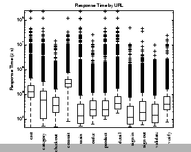
Figure 3 presents box plots depicting the response time distributions of the twelve main request classes in our PetStore testbed. Response times differ significantly for different types of requests, hence the request mix is quite versatile in its effect on the system.
We mimic key aspects of real-world workload, e.g., varying burstiness at fine time scales and periodicity on longer time scales. However, each experiment runs in 1-2 days, so the periods of workload variation are shorter than in the wild. We wrote simple scripts to generate session files for the httperf workload generator [28], which allows us to vary the client think time and the arrival rate of new client sessions.
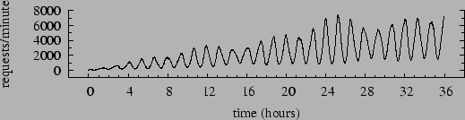
In this experiment we gradually increase the number of concurrent client sessions. We add an emulated client every 20 minutes up to a limit of 100 total sessions, and terminate the test after 36 hours. Individual client request streams are constructed so that the aggregate request stream resembles a sinusoid overlaid upon a ramp; this effect is depicted in Figure 4, which shows the ideal throughput of the system under test. The ideal throughput occurs if all requests are served instantaneously. Because httperf uses a closed client loop with think time, the actual rate depends on response time.
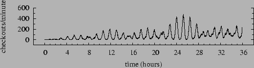
Each client session follows a simple pattern: go to main page, sign in, browse products, add some products to shopping cart, check out, repeat. Two parameters indirectly define the number of operations within a session. One is the probability that an item is added to the shopping cart given that it has just been browsed. The other is the probability of proceeding to the checkout given that an item has just been added to the cart. These probabilities vary sinusoidally between 0.42 and 0.7 with periods of 67 and 73 minutes, respectively. The net effect is the ideal time-varying checkout rate shown in Figure 5.
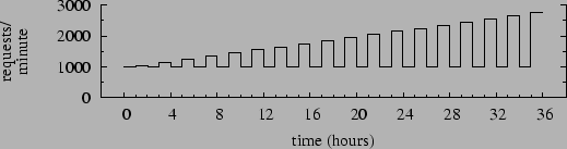
This 36-hour run has two workload components. The first httperf creates a steady background traffic of 1000 requests per minute generated by 20 clients. The second is an on/off workload consisting of hour-long bursts with one hour between bursts. Successive bursts involve 5, 10, 15, etc. client sessions, each generating 50 requests per minute. Figure 6 summarizes the ideal request rate for this pattern, omitting fluctuations at fine time scales.
The intent of this workload is to mimic sudden, sustained bursts of increasingly intense workload against a backdrop of moderate activity. Each ``step'' in the workload produces a different plateau of workload level, as well as transients during the beginning and end of each step as the system adapts to the change.
|
 |
BUGGY was a five-hour run with 25 client sessions. Aggregate request rate ramped from 1 request/sec to 50 requests/sec during the course of the experiment, with sinusoidal variation of period 30 minutes overlaid upon the ramp. The probability of add-to-cart following browsing an item and the probability of checkout following add-to-cart vary sinusoidally between 0.1 and 1 with periods of 25 and 37 minutes, respectively. This run occurred before the Petstore deployment was sufficiently tuned as described previously. The J2EE component generated numerous Java exceptions, hence the title ``BUGGY.''
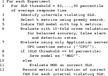
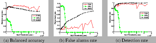
This section evaluates our approach using the system and workloads described in Section 4. In these experiments we varied the SLO threshold to explore the effect on the induced models, and to evaluate accuracy of the models under varying conditions. For each workload, we trained and evaluated a TAN classifier for each of 31 different SLO definitions, given by varying the threshold on the average response time such that the percentage of intervals violating the SLO varies from 40% to 10% in increments of 1%. As a baseline, we also evaluated the accuracy of the 60-percentile SLO classifier (MOD) and a simple ``rule of thumb'' classifier using application server CPU utilization as the sole indicator metric. Table 2 summarizes the testing procedure.
Table 3 summarizes the average accuracy of all models across all SLO thresholds for each workload. Figure 7 plots the results for all 31 SLO definitions for STEP. We make several observations from the results:
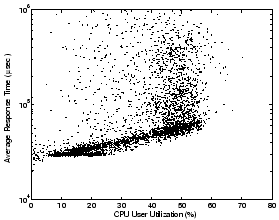 |
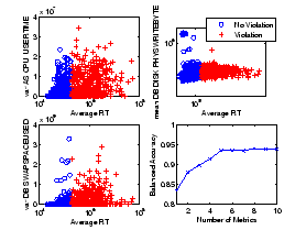
Determining the number of metrics. To illustrate the role of multiple metrics in accurate TAN models, Figure 9 shows the top three metrics (in order) as a function of average response time for the STEP workload with SLO threshold of 313 msec (20% instances of SLO violations). The top metric alone yields a BA score of 84%, which improves to 88% with the second metric. However, by itself, the second metric is not discriminative; in fact, the second metric alone yields a BA of just 69%. The TAN combines these metrics for higher accuracy by representing their relationships. Adding two more metrics increases the BA score to 93.6%.
 |
|
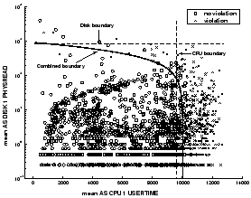
Interaction between metrics and values. The metrics selected for a TAN model may have complex relationships and threshold values. The combined model defines decision boundaries that classify the SLO state (violation/no violation) of an interval by relating the recorded values of the metrics during the interval. Figure 10 depicts the decision boundary learned by a TAN model for its top two metrics. The figure also shows the best decision boundary when these metrics are used in isolation. We see that the top metric is a fairly good predictor of violations, while the second metric alone is poor. However, the decision boundary of the model with both metrics takes advantage of the strength of both metrics and ``carves out'' a region of value combinations that correlate with SLO violations.
 |
Adaptation. Additional analysis shows that the models must adapt to capture the patterns of SLO violation with different response time thresholds. For example, Figure 7 shows that the metrics selected for MOD have a high detection rate across all SLO thresholds, but the increasing false alarm rate indicates that it may be necessary to adjust their threshold values and decision boundaries. However, it is often more effective to adapt the metrics as conditions change.
To illustrate, Table 4 lists the metrics selected for at least six of the SLO definitions in either the RAMP or STEP experiments. The most commonly chosen metrics differ significantly across the workloads, which stress the testbed in different ways. For RAMP, CPU usertime and disk reads on the application server are the most common, while swap space and I/O traffic at the database tier are most highly correlated with SLO violations for STEP. A third and entirely different set of metrics is selected for BUGGY: all of the chosen metrics are related to disk usage on the application server. Since the instrumentation records only system-level metrics, disk traffic is most highly correlated with the server errors occuring during the experiment, which are logged to disk.
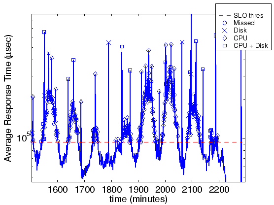
Metric ``Attribution''. The TAN models identify the metrics that are most relevant--alone or in combination--to SLO violations, which is a key step toward a root-cause analysis. Figure 11 demonstrates metric attribution for RAMP with SLO threshold set at 100msec (20% of the intervals are in violation). The model includes two metrics drawn from the application server: CPU user time and disk reads. We see that most SLO violations are attributed to high CPU utilization, while some instances are explained by the combination of CPU and disk traffic, or by disk traffic alone. For this experiment, violations occurring as sudden short spikes in average response time were explained solely by disk traffic, while violations occurring during more sustained load surges were attributed mostly to high CPU utilization, or to a combination of both metrics.
 |
Forecasting. Finally, we consider the accuracy of TAN models in forecasting SLO violations. Table 5 shows the accuracy of the models for forecasting SLO violations three sampling intervals in advance (sampling interval is 5 minutes for STEP and 1 minute for the others). The models are less accurate for forecasting, as expected, but their BA scores are still 80% or higher. Forecasting accuracy is sensitive to workload: the RAMP workload changes slowly, so predictions are more accurate than for the bursty STEP workload. Interestingly, the metrics most useful for forecasting are not always the same ones selected for diagnosis: a metric that correlates with violations as they occur is not necessarily a good predictor of future violations.
|
To further validate our methods, we analyzed data collected by a group of HP's OpenView developers on a different Web service testbed. The important characteristic of these tests is that they induce performance behaviors and SLO violations with a second application that contends for resources on the Web server, rather than by modulating the Web workload itself.
The testbed consists of an Apache2 Web server running on a Linux 2.4 system with a 600 MHz CPU and 256 MB RAM. The Web server stores 2000 files of size 100 KB each. Each client session fetches randomly chosen files in sequence at the maximum rate; the random-access workload forces a fixed portion of the requests to access the disk. This leads to an average response time for the system of around 70 msec, with a normal throughput of about 90 file downloads per second.
We analyzed data from four test runs, each with a competing ``resource hog'' process on the Web server:
We used a single SLO threshold derived from the system response time without contention. For each test the system learns a TAN model based on 54 system-level metrics collected using SAR at 15 second intervals. We omit detailed results for the CPU test: for this test the induced models obtained 100% accuracy using only CPU metrics. Table 6 summarizes the accuracy of the TAN models for the other three tests.
|
Table 7 shows the metrics selected for the TAN models for each test. We see that for the Memory and I/O bottleneck tests, the TAN algorithm selected metrics that point directly to the bottleneck. The metrics for the disk bottleneck experiment are more puzzling. One of the metrics is the one-minute average load (loadavg1), which counts the average number of jobs active over the previous minute, including jobs that have been queued waiting for I/O. Since disk metrics were not recorded in this test, and since the file operations did not cause any unusual CPU, network, memory or I/O load, this metric serves as a proxy for the disk queues. To pinpoint the cause of the performance problem in this case, it is necessary also to notice that CPU utilization dropped while load average increased. With both pieces of information one can conclude that the bottleneck is I/O-related.
These results provide further evidence that the analysis and TAN models suggest the causes of performance problems, either directly or indirectly, depending on the metrics recorded.
|
Jain's classic text on performance analysis [25] surveys a wide range of analytical approaches for performance modeling, bottleneck analysis, and performance diagnosis. Classical analytical models are based on a priori knowledge from human experts; statistical analysis helps to parameterize the models, characterize workloads from observations, or selectively sample a space of designs or experiments. In contrast, we develop methods to induce performance models automatically from passive measurements alone. The purpose of these models is to identify the observed behaviors that correlate most strongly with application-level performance states. The observations may include but are not limited to workload measures and device measures.
More recent books aimed at practitioners consider goals closer to ours but pursue them using different approaches. For example, Cockcroft & Pettit [12] cover a range of facilities for system performance measurement and techniques for performance diagnosis. They also describe Virtual Adrian, a performance diagnosis package that encodes human expert knowledge in a rule base. For instance, the ``RAM rule'' applies heuristics to the virtual memory system's scan rate and reports RAM shortage if page residence times are too low. Whereas Virtual Adrian examines only system metrics, our approach correlates system metrics with application-level performance and uses the latter as a conclusive measure of whether performance is acceptable. If it is, then our approach would not report a problem even if, e.g., the virtual memory system suffered from a RAM shortage. Similarly, Virtual Adrian might report that the system is healthy even if performance is unacceptable. Moreover, we propose to induce the rules relating performance measures to performance states automatically, to augment or replace the hand-crafted rule base. Automatic approaches can adapt more rapidly and at lower expense to changes in the system or its environment.
Other recent research seeks to replace human expert knowledge with relatively knowledge-lean analysis of passive measurements. Several projects focus on the problem of diagnosing distributed systems based on passive observations of communication among ``black box'' components, e.g., processes or Java J2EE beans implementing different tiers of a multi-tier Web service. Examples include WebMon [20], Magpie [4], and Pinpoint [10]. Aguilera et. al. [2] provides an excellent review of these and related research efforts. It also proposes several algorithms to infer causal paths of messages related to individual high-level requests or transactions, and to analyze the occurrences of those paths statistically for performance debugging. Our approach is similar to these systems in that it relates application-level performance to hosts or software components as well as physical resources. The key difference is that we consider metrics collected within hosts rather than communication patterns among components; in this respect our approach is complementary.
Others are beginning to apply model-induction techniques from machine learning to a variety of systems problems. Mesiner et. al. [27], for instance, apply decision-tree classifiers to predict properties of files (e.g., access patterns) based on creation-time attributes (e.g., names and permissions). They report that accurate models can be induced for this classification problem, but that models from one production environment may not be well-suited to other environments; thus an adaptive approach is necessary.
TANs and other statistical learning techniques are attractive for self-managing systems because they build system models automatically with no a priori knowledge of system structure or workload characteristics. Thus these techniques--and the conclusions of this study--can generalize to a wide range of systems and conditions. This paper shows that TANs are powerful enough to capture the performance behavior of a representative three-tier Web service, and demonstrate their value in sifting through instrumentation data to ``zero in'' on the most relevant metrics. It also shows that TANs are practical: they are efficient to represent and evaluate, and they are interpretable and modifiable. This combination of properties makes TANs particularly promising relative to other statistical learning approaches.
One focus of our continuing work is online adaptation of the models to respond to changing conditions. Research on adapting Bayesian networks to incoming data has yielded practical approaches [22,6,19]. For example, known statistical techniques for sequential update are sufficient to adapt the model parameters. However, adapting the model structure requires a search over a space of candidate models [19]. The constrained tree structure of TANs makes this search tractable, and TAN model induction is relatively cheap. These properties suggest that effective online adaptation to a continuous stream of instrumentation data may well be feasible. We are also working to ``close the loop'' for automated diagnosis and performance control. To this end, we are investigating forecasting techniques to predict the likely duration and severity of impending violations; a control policy needs this information to balance competing goals. We believe that ultimately the most successful approach for adaptive self-managing systems will combine a priori models (e.g., from queuing theory) with automatically induced models. Bayesian networks--and TANs in particular--are a promising technology to achieve this fusion of domain knowledge with statistical learning from data.
tex2html_bgroup
This document was generated using the LaTeX2HTML translator Version 2002 (1.62)
Copyright © 1993, 1994, 1995, 1996,
Nikos Drakos,
Computer Based Learning Unit, University of Leeds.
Copyright © 1997, 1998, 1999,
Ross Moore,
Mathematics Department, Macquarie University, Sydney.
The command line arguments were:
latex2html -split 0 -show_section_numbers -local_icons paper.tex
The translation was initiated by Jeff Chase on 2004-10-06
|
This paper was originally published in the
Proceedings of the 6th Symposium on Operating Systems Design and Implementation,
December 6–8, 2004, San Francisco, CA Last changed: 18 Nov. 2004 aw |
|
![$\displaystyle \sum_i \log [\frac{P(m_i\vert m_{p_i},s^-)}{P(m_i\vert m_{p_i},s^+)}] + \log
\frac{P(s^-)}{P(s^+)} > 0$](img39.png)