| Pp. 121–128 of the Proceedings |  |
Dr. John A. Board
Duke University
jab@ee.duke.edu
https://www.ee.duke.edu/~jab
Also of increasing research interest is the subject of Cluster Computing. These clusters of workstations are capable of achieving the performance of traditional supercomputers (on certain problems) at a significantly reduced cost. Such clusters are often loosely coupled groups of machines which communicate using commodity networking hardware. Networking is often 100 Mb/s ethernet, although 1 Gb/s ethernet and proprietary solutions such as Myrinet are becoming more common.
Unfortunately, while there exist many vendor implementations of high speed parallel FFTs for tightly coupled traditional supercomputers, there are few parallel implementations available for clusters of workstations. In our work, we had a need for a portable and efficient parallel FFT. Not finding one that fit both of our criteria, we decided to implement our own. It was found that the use of this parallel FFT in our code allowed for a great deal of improvement in its performance.
Other researchers, when facing this problem, have resorted to using a naive DFT. So long as one is willing to have multiple processors each keep a copy of the space upon which the DFT is to be performed, the DFT is highly scalable in that the results for any given point in the space do not depend on earlier computation that may have been performed on another processor. While this approach can achieve not only speed up, but also performance improvements over a serial FFT, it seems aesthetically unpleasing and if an efficient, portable, parallel FFT is available, it might not be the best use of processor resources.
The latest versions of the FFTW library do have a parallel FFT using MPI for interprocess communications. While our application (DPME) is written using PVM, this would not have been a serious impediment as we were already considering an MPI port of DPME. Unfortunately, the FFT did not scale for problem sizes we are interested in (except for very large FFTs, 256x256x256, the speedup was less than 1). This was even true when using the "transposed" FFT which has significantly less communication (see below for a discussion of transposed FFTs).
Each slab of the data space contains (for now, exactly) m = N/P
2D slices. Each processor computes a single 2D FFT on each of
its m slices, sending the results to all other processors using
non-blocking communication. After each processor has received all of
the data sent to it, the data is scattered on the processors as seen
in Figure 2.
Finally, each processor performs m*N 1D FFTs in the final dimension,
yielding the 3D FFT. Note that unless an additional communication
step is performed, the resulting data is on different processors than
was the original data. This is known as a transposed FFT. In this
case, performing either a forwards or backwards FFT results in the
Most Significant and the Second Most Significant axes being swapped.
So, if the original data layout was stored in ZYX major order, with
the data along the Z axis being partitioned to different processors,
either a forwards or backwards FFT would result in a changed data
layout to YZX major order with the Y axis partitioned to the different
processors. The algorithm was designed this way in order to minimize
communication, while still being symmetric. In other words, one may
call the forward or backward FFT first and have the opposite call put
the data back in place.
No kernel patches have been applied to increase network performance as
it was found that machines were already capable of 95% of wire speed
bandwidth. Kernel patches designed to reduce latency might increase
performance slightly at the cost of reducing cluster maintainability.
The parallel programming of this cluster has been performed using both
PVM and MPI. PVM ([GBD+94]) results are given using version 3.4.3.
MPI ([SOHL+96]) results were found using LAM MPI version 6.3.1.
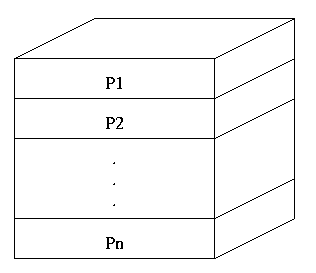
Figure 1: Processor representation of the 3D data space
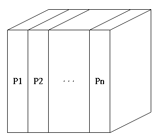
Figure 2: Processor representation of the 3D data space after 2D FFTs and communication step.
Testbed Configuration
All of the experimental results given in this paper were computed on a
cluster of 16 dual processor machines. The processors are Intel Pentium
II running at a clock speed of 450 MHz. Each node has 512 MB of RAM
as well as an additional 512 MB of virtual memory. The machines are
connected using a private 100 Mb/s Ethernet Cisco 2924 switch. All nodes
are running the GNU/Linux operating system with kernel release 2.2.12
compiled for SMP. FFT Results
The FFT algorithm described above performs very well provided that
one can make use of transposed data in Fourier space. Fortunately,
DPME's computation of the electrostatic potential in Fourier space can
easily accommodate transposed data. Speed-up results (as compared
to a single call to the sequential FFTW 3D FFT routine) for this
algorithm are given in Figure 3 and Figure 5
(Figure 4 and Figure 6 give the respective timings).
As can be seen from the figures, the method achieves reasonable efficiency
for up to 12 processors. The sudden degradation after 12 processors in
performance will be discussed in a subsequent section.
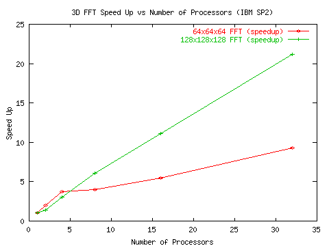
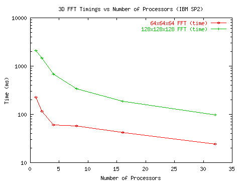
The algorithm has also been tested on the IBM SP2 at the North Carolina Super-Computing Center (NCSC). As shown in Figure 7 and Figure 8, the algorithm exhibits moderate speed-up for small FFTs (64x64x64) and good speed-up for medium sized FFTs (128x128x128) - 70% efficiency for up to 32 processors.


Figure 4: 3D FFT performance on the Duke ECE Beowulf Cluster - timings

Figure 5: 3D FFT performance on the Duke ECE Beowulf Cluster - speedup

Figure 6: 3D FFT performance on the Duke ECE Beowulf Cluster - timings
At the time, the cluster used an Intel 510T 100 Mb/s switch. It was decided to try replacing this switch with a Cisco 2924. After the replacement, we saw improved scalability of the FFT algorithm up to 12 processors. These results were well correlated with those presented by Mier Communications, Inc ([Mie98]) for the number of simultaneous 100 Mb/s full-duplex streams that could be supported by the various switches without dropping packets. It should be noted that the Mier results were for the Cisco 2916 and the Intel 510T. However, the Cisco 2916 and 2924 have similar backplane architectures.
The Mier Communications tests also included a comparison with the Bay 350. We then tried using a switch in the same family, the Bay 450. Again, the scaling results on our algorithm were well correlated with the number of simultaneous 100 Mb/s full-duplex streams that the switch backplane could handle without dropping packets.
It is uncertain why the switches perform so differently. The backplanes of each switch are all rated at over 2 Gb/s (Intel - 2.1 Gb/s, Bay - 2.5 Gb/s, Cisco - 3.2 Gb/s). Latency also does not appear to be a factor as all of the switches have minimum latency times of 10us or less. The most likely reason behind the differences is that the backplane architecture of the various switches results in the Intel switch dropping packets under full load. Since MPI and PVM communicate using TCP/IP protocols, this results in the packet being resent.
Therefore, the strong correlation between the number of simultaneous full-duplex streams (found by Mier) and our own scaling results is likely due to the nature of our algorithm which aims to fully utilize the switch architecture by having each processor send data to every other processor after each 2D slice of the data has been converted to Fourier space. So, each processor is not only sending data to all other processors, but is also receiving data from each of the other processors. The amount of data in each message depends on the size of the FFT and the number of processors being utilized. In general, it is: B * N2 / P where B is the data size (for the complex doubles we are using, this is 16 bytes), N is the size along one dimension of the FFT and P is the number of processors. For a 64x64x64 FFT on 4 processors, the messages are 16 kB in size. The number of messages is N * P. The number and size of these messages insures that the switch is fully utilized on the P ports. Therefore, the number of simultaneous full-duplex streams capable of being supported is very important.
Determining whether the most important factor in the algorithm's performance is the switch bandwidth or the overall latency is a fairly difficult task. The various switches we used on our local cluster all had similar latencies and had the same (theoretical bandwidths), however, they performed in vastly different manners. The IBM SP2 had a completely different switch architecture, with over 1 Gb/s bandwidth and very low latencies. However, some analysis of the amount of data being sent should give us some idea of which factor (bandwidth or latency) is the most important.
Consider a 64x64x64 parallel 3D FFT running on 4 processors. Each 2D slice of the data is 64 kB in size. Each message (to the 3 other processors) for this slice is 16 kB in size. On a 100 Mb/s switch, the theoretical minimum time that this message could cross the network is approximately 1.3ms. Switch latencies are on the order of 10us. When the TCP stack latencies are considered, the latencies involved are still roughly an order of magnitude less than the time to transfer the message. Of course if more processors are used, if the FFTs are smaller, or if the switch bandwidth increases, the latencies inherent in the switch and the TCP stack become significantly more important.
This fact has been recognized by IBM in developing the SP2 in that there are two interfaces for accessing the switch. The standard method routes a user's network requests through the kernel to the adapter and then to the switch. This results in a throughput of 440 Mb/s primarily because of the latency of 165us. The second method bypasses the kernel and goes directly from user space to the adapter, resulting in the throughput increasing by a factor of 2.4 to approximately 1 Gb/s due in part to the latency being decreased by a factor of 6.9 to 24us. If we repeat the previous examination of bandwidth versus latency for the two SP2 network interfaces, on the first interface we find that at a speed of 440 Mb/s, each message only requires 297us to traverse the switch. In this case, the 165us latency is within the same order of magnitude as the transport time, causing latency to be a much greater factor than for our 100 Mb/s switches. For the second interface, the transport time is 123us while the latency is 24us. So, on the SP2 we see that latency is more important primarily because of the maximum speed of the switch itself.

Due to the periodic boundary conditions, the reciprocal sum is a set of N periodic functions. By solving this problem in the Fourier domain, the infinite periodic functions converge rapidly. The result can then be converted back into real space and summed with the direct space results to obtain the electrostatic potential for the original problem space.
To solve the reciprocal sum, one first discretizes the problem space as a 3D mesh. The charge functions are then interpolated onto the mesh. A 3D FFT is then performed on the mesh, transforming it into Fourier space. The electrostatic potential of the the mesh is computed (still in Fourier space). The mesh is transformed back into real space (by means of an inverse FFT). Finally, the electrostatic potentials of the original point charge locations are interpolated, based on the values in the 3D mesh.
The direct and reciprocal space electrostatic potentials can then be summed to find the electrostatic potential of the total problem space at the locations of each point charge. As was previously mentioned, solving the direct space portion of the problem is O(N). The reciprocal sum's order of complexity is: O(M log2(M) + p3 * M) where p is the order of interpolation when converting to or from the mesh and M is the number of mesh points. The 3D FFT is O(M log2 (M)) and the interpolation is O(p3 * M). If M is approximately N, then the complexity of PME is O(N log2(N)).
DPME uses a Master/Slave model for performing parallel computations. The direct sum is performed on the set of Slave processors spawned by PVM. The Master processor performs the reciprocal sum serially. This decision was primarily made due to the lack of a parallel FFT with a speed-up greater than 1 for a cluster of workstations.
DPME has several options which affect performance. The most significant of these is the Ewald Parameter (a) which is inversely proportional to the width of the Gaussian charge distribution. By adjusting the width of the Gaussian, one can shift work between the direct sum and the reciprocal sum. For example, a very narrow Gaussian charge distribution would allow for a small cut-off radius in the direct sum without incurring a large error penalty. However, a narrow Gaussian distribution would require a large number of mesh points in the reciprocal sum. Conversely, a wide charge distribution would result in a nearly uniform reciprocal sum and would therefore require few mesh points, however, the cut-off radius would have to be proportionally larger.
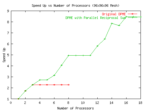
Since the reciprocal sum in DPME is sequential, the obvious strategy to increase its scalability is to set the Ewald parameter relatively small (a wider Gaussian charge distribution). This places most of the work in the direct sum which has a great deal of scalability. Unfortunately, there is a limit to how wide the charge distribution can be. If it is too wide, then the work in the direct sum approaches O(N2) complexity minimizing the advantages of using a larger number of processors. In general, it was found that optimal performance was achieved using 8 direct sum processors along with the 1 reciprocal sum processor. However, these results were obtained on an older generation of processors. On the cluster we are currently developing under, the performance was significantly worse (see Figure 10).


The FFT itself is general purposed and unlike much other work in the field, it will achieve reasonable speed up on a cluster of workstations. It should give some hope to people contemplating the massively scalable DFT as a replacement for FFT code.
Another place where the FFT code might be optimized is in the amount of work done per communication call. As our algorithm stands now, each 2D slice of the data has a 2D FFT performed on it and it is then divided and sent to all other processors. It might prove to be more efficient to perform multiple 2D FFTs before sending the data to the other processors. Of course, if all slices were computed before sending the data, then our algorithm would be identical to the FFTW parallel algorithm. However, there may be an optimal point somewhere between 1 and all slices at a time.
|
This paper was originally published in the
Proceedings of the 4th Annual Linux Showcase and Conference, Atlanta,
October 10-14, 2000, Atlanta, Georgia, USA
Last changed: 8 Sept. 2000 bleu |
|