A Formal Model of Provenance in Distributed Systems
Issam Souilah
University of Southampton, UK
Adrian Francalanza
University of Malta, Malta
Vladimiro Sassone
University of Southampton, UK
We present a formalism for provenance in distributed systems based on
the  -calculus. Its main feature is that all data products are
annotated with metadata representing their provenance. The calculus is
given a provenance tracking semantics, which ensures that data
provenance is updated as the computation proceeds. The calculus also
enjoys a pattern-restricted input primitive which allows processes to
decide what data to receive and what branch of computation to proceed
with based on the provenance information of data. We give examples to
illustrate the use of the calculus and discuss some of the semantic
properties of our provenance notion. We conclude by reviewing related
work and discussing directions for future research.
-calculus. Its main feature is that all data products are
annotated with metadata representing their provenance. The calculus is
given a provenance tracking semantics, which ensures that data
provenance is updated as the computation proceeds. The calculus also
enjoys a pattern-restricted input primitive which allows processes to
decide what data to receive and what branch of computation to proceed
with based on the provenance information of data. We give examples to
illustrate the use of the calculus and discuss some of the semantic
properties of our provenance notion. We conclude by reviewing related
work and discussing directions for future research.
As a concept, provenance indicates the source and derivation of an
object, and is also known as origin, lineage and pedigree. More
concretely, provenance refers to a record of such source and
derivation [19]. This record may include information
about the ownership, influences, contributions and any other
historical or contextual information which may be deemed
relevant and useful. Provenance has many applications such as auditing,
detecting errors and ensuring reproducibility of results. It is also
central to the trust one places in data, since it can be used as
an indicator of quality, especially in a setting where independent
verification of other attributes may not be possible.
Provenance tracking is the problem of recording provenance information,
and has been studied in a wide range of settings, including databases
[4,8,11,5,7],
scientific computing
[13,21,12,22]
and file systems [20]. Initially, most of the
work on provenance relied on intuitive and informal concepts such as
influences, contributes to, and depends on in
defining what provenance means. These notions were then used to provide
mostly ad hoc implementations, with no formal guarantees as to their
correctness or adequacy. However, lately there have been a surge of
interest in underpinning the more theoretical principles of provenance
[4,11,7]. Such body of work aims
to establish a mathematical and semantic basis for provenance, which is
important if we are to compare different notions of provenance and
assess the correctness of their implementations. The present work falls
in this latter line of research and aims to provide a formal study of
provenance-based trust in concurrent and distributed systems.
We choose the asynchronous -calculus
[15,3], a version of the -calculus
[18] where message output is non-blocking, as the
formalism for modelling distributed systems. The choice of asynchrony is
motivated mainly by the envisaged applications of our calculus and its
impact on possible implementations, however, it has minimal effect on
our results. In order to be able to refer to individual agents, we
extend this basic formalism with explicit identities. These identities
can be thought of as representing units of trust, and are merely
labels for identifying processes with no effect on communication (cf. localities in the DPI calculus [14]). With
this extension we can express the essence of computation in a
distributed setting, whereby multiple agents interact by exchanging
messages. For instance the code:
denotes a system composed of three principals:  and
and  that are
sending values
that are
sending values  and
and  on the same channel
  and
and  that is
attempting to read a value from the channel and use it in the
continuation code
that is
attempting to read a value from the channel and use it in the
continuation code  . Interestingly, from the point of view of ,
there exists a level of non-determinism, that is a market of
values on channel from which is free to choose. However,
assuming has no way of assessing the quality of the different
values available on channel , it cannot decide which of the two
values or to consume. In such situations, provenance
may be used as a measure of the quality of data. For example, the three
principals may agree on a convention whereby the senders (producers of
data) attach a provenance tag. Thus the code may be modified to:
. Interestingly, from the point of view of ,
there exists a level of non-determinism, that is a market of
values on channel from which is free to choose. However,
assuming has no way of assessing the quality of the different
values available on channel , it cannot decide which of the two
values or to consume. In such situations, provenance
may be used as a measure of the quality of data. For example, the three
principals may agree on a convention whereby the senders (producers of
data) attach a provenance tag. Thus the code may be modified to:
Now, the consumer of the data, , can determine where the data
originated from and branch accordingly. Even though this encoding works,
it carries two major disadvantages:
![\begin{inparaenum}[\itshape\upshape (1\upshape )]
\item it is cumbersome and mud...
...ere to these provenance conventions,
which cannot be enforced.
\end{inparaenum}](img11.png)
Crucially, the second point leads to circular reasoning with respect to
trust. For instance, in the above code nothing stops principal from
forging 's identity using
![$ b[n \langle a,v_2\rangle ]$](img12.png) . This simple
problem may be solved using a digital signature scheme for example,
however, in general the picture can be far more complicated as messages
may carry, not only data authored by the agent itself, but also data
obtained from other agents. Moreover, agents may consult other agents
about where to get data from and what to do with it. These may also be
of interest to consumers of data in order to be able to judge the
trustworthiness of data.
. This simple
problem may be solved using a digital signature scheme for example,
however, in general the picture can be far more complicated as messages
may carry, not only data authored by the agent itself, but also data
obtained from other agents. Moreover, agents may consult other agents
about where to get data from and what to do with it. These may also be
of interest to consumers of data in order to be able to judge the
trustworthiness of data.
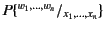
A distinguishing feature of our distributed -calculus extension is
the use of provenance annotated data. Every value,  , is
annotated with its provenance,
, is
annotated with its provenance,  , and denoted as
 . The provenance is a sequence of
`
. The provenance is a sequence of
` '-delimited events. The events in a provenance sequence
 are chronologically ordered with
  being the most recent event. An event
  may be an output event
 , which says that the value has been sent by an
agent on a channel whose provenance is , or an input event
, which says that the value has been sent by an
agent on a channel whose provenance is , or an input event
 , which says that the value has been received by
an agent on a channel whose provenance is ; the rationale
here is that in the -calculus channels are data too.
, which says that the value has been received by
an agent on a channel whose provenance is ; the rationale
here is that in the -calculus channels are data too.
We propose a two-tiered framework which automates the process of
provenance tracking and separates it from the actual
computation.1 This two-tiered framework is manifested by the provenance
tracking reduction semantics, which, in addition to describing the
interaction between agents, keeps the provenance of values up-to-date.
For instance, the rule for sending data on a particular channel has two
facets:
From the computational perspective, the rule represents the first of a
two-step communication process: a principal wanting to output a
value
 on a channel
 generates a packaged message
 , where
  represents the address and
 the annotated data content. From the provenance tracking
perspective, the rule also describes how the provenance of the value
is updated to
the annotated data content. From the provenance tracking
perspective, the rule also describes how the provenance of the value
is updated to
 after the
output operation. This tells us that the value has been most recently
sent by agent on a channel whose provenance is
after the
output operation. This tells us that the value has been most recently
sent by agent on a channel whose provenance is
 .
.
Dually, the rule for receiving values, the second step in communication,
has two facets as well:
![$\displaystyle \inference{\kappa_v \models \pi}{
b[m\mathord{:}\kappa_{m} (
\pi...
... \rangle\!\rangle
\rightarrow
b[P\{^{v\colon b?\kappa_m ;\kappa_v }/_{x}\}]
}
$](img30.png)
On the one hand, the rule states that principal can input a value
from channel and proceed as if there exists a packaged value
with destination in the system; otherwise it blocks until such a
packaged value becomes available. More importantly though, this rule
also describes how the provenance information attached to the packaged
data,  , is first used for vetting purposes before consumption,
and afterwards updated. More specifically, the data input on channel
only progresses if the provenance of the packaged data, ,
passes the input test ; this is denoted as
, is first used for vetting purposes before consumption,
and afterwards updated. More specifically, the data input on channel
only progresses if the provenance of the packaged data, ,
passes the input test ; this is denoted as
 .
Should this test succeed, the input is allowed to occur and, in
addition, the provenance attached to value is updated to
.
Should this test succeed, the input is allowed to occur and, in
addition, the provenance attached to value is updated to
 in the continuation
, thereby recording the fact that the value was received by principal
on some channel with provenance
in the continuation
, thereby recording the fact that the value was received by principal
on some channel with provenance  .
.
In addition to proposing a provenance-based calculus, we also formalise
a notion of correctness for our provenance annotations. We
interpret the provenance of an annotated value
as a partial order of assertions about
events that occurred in the system, relating specifically to
value . For example, the provenance of annotated value
tells us that
has been sent by principal on some channel with provenance
, and that before this, the events described by
and
 took place, without restricting the relative ordering
between the events in
and
; the information in
the recorded event
took place, without restricting the relative ordering
between the events in
and
; the information in
the recorded event
 is also partial because it
does not specify the channel on which was sent. To prove
correctness, we devise a technique whereby a decorated version of our
reduction semantics constructs a global log which records a total
ordering of past events relating to all values. The provenance
of an annotated value is then correct if its partial order denotation
is, in some sense, consistent with the total ordering of events
specified by the global log.
is also partial because it
does not specify the channel on which was sent. To prove
correctness, we devise a technique whereby a decorated version of our
reduction semantics constructs a global log which records a total
ordering of past events relating to all values. The provenance
of an annotated value is then correct if its partial order denotation
is, in some sense, consistent with the total ordering of events
specified by the global log.
The rest of the paper is structured as follows. In
§2, we give an overview of the calculus, review
its syntax and semantics, and provide examples to illustrate some of its
features. We discuss what past information is exactly recorded by the
provenance tracking reduction relation and study its correctness properties
in §3. In §4, we
review related work. In §5, we discuss
possibilities for future work and conclude the paper.
2 The Provenance Calculus
The formalism we consider for studying provenance is a variant of the
asynchronous -calculus, which we extend with the following four
main features:
- Explicit identities: every process is located at a
named principal, which is used for provenance and
does not otherwise affect communication between processes.
- Annotated data: every value is annotated with its
provenance, which is updated as the computation
proceeds to reflect what happened to the value.
- Provenance tracking: we specify the meaning of the
calculus by a provenance tracking reduction semantics which,
in addition to describing the possible interactions between
principals, also tracks the provenance of values as they are exchanged
between principals.
- Pattern restricted input: In order to allow principals to
make use of the provenance information of values, we adopt a version
of guarded choice that is restricted to inputs on the same channel
with possibly differing patterns (similar in spirit to the one used
in [6]). This allows principals to
restrict the set of values they are willing to receive on a particular
channel to those that satisfy the patterns specified. It also allows
them to branch to different continuations based on the provenance
information.
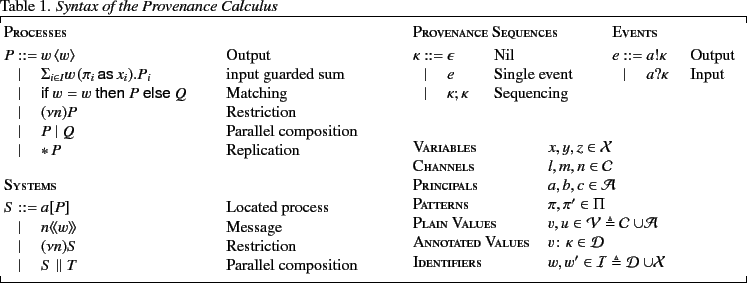
The formal syntax of the calculus is given in Table 1. We
assume a set
 of variables, ranged over by
 , a set
 of channel names, ranged over
by
of channel names, ranged over
by
 , and a set
 of principal names,
ranged over by
of principal names,
ranged over by
 . We assume that all three sets are
pair-wise disjoint and define the set
. We assume that all three sets are
pair-wise disjoint and define the set
 of plain
values to be
of plain
values to be
 , and use the letters
 to range over this set.
We represent provenance as a sequence of events. The events in a
provenance sequence are assumed to be temporally ordered from left to
right, where the left-most event (the head of the sequence) is the most
recent event. We use
 for the set of provenance sequences
and
for the set of provenance sequences
and
 for the set of events and let
 and
and
 range over elements of each set
respectively.
range over elements of each set
respectively.
The set
 of annotated values is then defined to be
the set of terms of the form
where is a plain
value and its provenance. An output event
in the provenance of a value denotes that the
value has been sent by principal on a channel whose provenance is
, while an input event denotes that the
value has been received by principal on a channel whose provenance
is . We also define the set
of annotated values is then defined to be
the set of terms of the form
where is a plain
value and its provenance. An output event
in the provenance of a value denotes that the
value has been sent by principal on a channel whose provenance is
, while an input event denotes that the
value has been received by principal on a channel whose provenance
is . We also define the set
 of identifiers to be
 and let
 range over
identifiers.
range over
identifiers.
To allow principals to query the provenance of values we use patterns
and pattern matching. Instead of defining a particular pattern
matching language, we opt for a more general approach and make the
calculus parametric on the choice of the pattern matching language. We
do give a concrete language to use with the examples however.
Definition 1
A pattern matching language is a pair

where

is
a set of patterns, ranged over by

, and

is the pattern
satisfaction (or matching) relation, a relation between provenance
sequences and patterns.
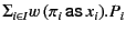
Processes in our calculus are based on those of the asynchronous
-calculus and are ranged over by
 . The main
differences with respect to the asynchronous -calculus is our use
of variants of the input and summation constructs. For input, we use a
variant that takes two parameters in the form
. The main
differences with respect to the asynchronous -calculus is our use
of variants of the input and summation constructs. For input, we use a
variant that takes two parameters in the form
 ,
where is a pattern that is used to restrict the set of values to
be received to those whose provenance matches the pattern and
,
where is a pattern that is used to restrict the set of values to
be received to those whose provenance matches the pattern and  is the standard variable binder, a placeholder for the value to be
received. We use the notation
is the standard variable binder, a placeholder for the value to be
received. We use the notation
 for the process
that is ready to receive, on channel
for the process
that is ready to receive, on channel  , a value whose provenance
matches the pattern and continue as with the appropriate
substitution. For summation, we use a restricted version that only
allows input guarded choice on the same channel, denoted by
, a value whose provenance
matches the pattern and continue as with the appropriate
substitution. For summation, we use a restricted version that only
allows input guarded choice on the same channel, denoted by
 for some finite index set
  .
We use the notation 0 as syntactic sugar for the empty sum. The output
form
.
We use the notation 0 as syntactic sugar for the empty sum. The output
form
 denotes the process that is ready to send
  on
channel , while
on
channel , while
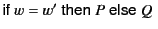 denotes the process that
proceeds as if is equal to and as
denotes the process that
proceeds as if is equal to and as  otherwise. Scope
restriction of channel to process is denoted by
otherwise. Scope
restriction of channel to process is denoted by
 . Parallel composition of processes and is
denoted by
. Parallel composition of processes and is
denoted by  while
while
 denotes replication of process
. It should be noted that all values in processes are annotated
values, except channel names in restrictions. The reason for that is
that we use restriction as usual to delimit scope, yet within one scope
a channel name may have occurrences with possibly different provenance
sequences.
denotes replication of process
. It should be noted that all values in processes are annotated
values, except channel names in restrictions. The reason for that is
that we use restriction as usual to delimit scope, yet within one scope
a channel name may have occurrences with possibly different provenance
sequences.
A system is the composition of zero or more located
processes and messages. We use
 to range over
systems. A located process,
to range over
systems. A located process, ![$ a[P]$](img73.png) , is a process that is
running under the authority of a principal . We overload the symbol
0 to denote the located process
, is a process that is
running under the authority of a principal . We overload the symbol
0 to denote the located process ![$ a[0]$](img74.png) . As the structure of our
systems is flat, it should be obvious from the context whether we mean
by 0 the empty summation or the located process . A
message is a value that has been sent but not yet received, and is
denoted in the calculus by
. As the structure of our
systems is flat, it should be obvious from the context whether we mean
by 0 the empty summation or the located process . A
message is a value that has been sent but not yet received, and is
denoted in the calculus by
 .
Restriction is denoted by
.
Restriction is denoted by  while parallel composition
of two systems is denoted by
while parallel composition
of two systems is denoted by
 .
.
The semantics of the calculus is defined by two relations, the
structural congruence relation,  , and the
provenance tracking reduction relation,
, and the
provenance tracking reduction relation,
 . Structural
congruence allows us to make structural manipulations of systems
which makes the definition of reduction simpler. The structural
congruence relation is standard and is omitted due to space limitations.
. Structural
congruence allows us to make structural manipulations of systems
which makes the definition of reduction simpler. The structural
congruence relation is standard and is omitted due to space limitations.
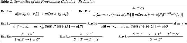
Interaction between located processes is described by the reduction
relation
. As we mentioned previously, the reduction relation
also tracks and updates the provenance of values as the system evolves.
The reduction relation is defined on closed systems (i.e., those
that contain no free variables) and is given in Table
2. The two main reduction rules are RED SND
and RED RCV, which describe sending and receiving values
respectively. The reason we split communication into the two steps of
sending and receiving is to make the semantics simpler by only adding a
single event to the provenance sequence at a time. In the rule
RED SND, a located process
![$ a[m\mathord{:}\kappa_{m} \langle v\colon\kappa_{v}\rangle ]$](img81.png) may output
the value
on the channel
which results in the message
. What should be noted here is that the provenance of
the value changes from
to
after the output action to reflect the fact that the
value has been most recently sent by principal on a channel whose
provenance is
. In the rule RED RCV, a message
may output
the value
on the channel
which results in the message
. What should be noted here is that the provenance of
the value changes from
to
after the output action to reflect the fact that the
value has been most recently sent by principal on a channel whose
provenance is
. In the rule RED RCV, a message
 may be received by the located process
![$ a[\Sigma_{i \in I}m\colon\kappa_{m} (
\pi_{i} \mathsf{as} x_{i}).P_{i}]$](img83.png) if the provenance of the value satisfies one of the
patterns
if the provenance of the value satisfies one of the
patterns  . The process
  whose pattern
  is
satisfied is chosen for the continuation. If more than one such pattern
exists, one of them is chosen non-deterministically. Note that here too,
the provenance of the value is updated from to
is
satisfied is chosen for the continuation. If more than one such pattern
exists, one of them is chosen non-deterministically. Note that here too,
the provenance of the value is updated from to
 to reflect the fact that it has
most recently been received by principal on a channel with
provenance
. The value with the updated provenance is then
substituted for the variable in the continuation chosen. The capture
avoiding substitution of
to reflect the fact that it has
most recently been received by principal on a channel with
provenance
. The value with the updated provenance is then
substituted for the variable in the continuation chosen. The capture
avoiding substitution of
 for the free occurrences of
variables
for the free occurrences of
variables
 in is denoted by
 and its definition is standard. We let
 range over substitutions. The rules
 and
and
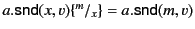
 give the semantics of matching. It should be
noted here that only the plain values are tested for equality while
their provenance is ignored.2 This means that if the two plain values are
equal, irrespective of their provenances, the process in the
then branch is chosen for the continuation as indicated by the
rule
. If the two plain values are not equal, then the
process in the else branch is chosen for the continuation as
indicated by the rule
. The other three rules are
standard and state that reduction is preserved under restriction, system
composition as well as under structural congruence.
give the semantics of matching. It should be
noted here that only the plain values are tested for equality while
their provenance is ignored.2 This means that if the two plain values are
equal, irrespective of their provenances, the process in the
then branch is chosen for the continuation as indicated by the
rule
. If the two plain values are not equal, then the
process in the else branch is chosen for the continuation as
indicated by the rule
. The other three rules are
standard and state that reduction is preserved under restriction, system
composition as well as under structural congruence.
In this section, we will give a few examples to illustrate the use of
the provenance calculus. First, however, we have to give a concrete
pattern matching language.
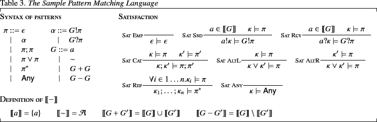
2.3.1 A Sample Pattern Matching Language
As our provenance sequences have a structure that is similar to that of
XML documents, we choose to base our sample pattern language on regular
expression pattern matching [16]. The formal syntax and
semantics of the language is given in Table 3.
The pattern
 matches any provenance sequence while the pattern
 is used to match the empty provenance sequence (denoted by
as well). The two patterns
is used to match the empty provenance sequence (denoted by
as well). The two patterns  and
and
 match send and receive events respectively. The use
of group expressions
match send and receive events respectively. The use
of group expressions  in these patterns allows us to perform
more general tests against the principal that performed the event. The
group expression denotes the singleton set containing principal
only, while
in these patterns allows us to perform
more general tests against the principal that performed the event. The
group expression denotes the singleton set containing principal
only, while
 denotes the set of all principals.
  and
and
 denote union and difference of groups respectively. The
denotation of group expressions is given by the function
denote union and difference of groups respectively. The
denotation of group expressions is given by the function
 . The pattern
  matches a provenance
sequence that is composed of two parts that match and
matches a provenance
sequence that is composed of two parts that match and  respectively. The alternation of patterns and , denoted
by
respectively. The alternation of patterns and , denoted
by
 , matches a sequence that matches either patterns,
while the repetition of pattern , denoted by
, matches a sequence that matches either patterns,
while the repetition of pattern , denoted by  , matches any
provenance sequence that is the composition of zero or more
sub-sequences, each of which matches the pattern .
, matches any
provenance sequence that is the composition of zero or more
sub-sequences, each of which matches the pattern .
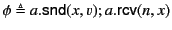
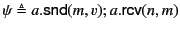
Provenance can be used to establish the
authenticity of messages, for example by checking their immediate
sender, their original sender or any principal in between. The following
system illustrates this.
In the above example, principal wants to receive only data coming
from directly, no matter where it has been before, whereas principal
wants to receive data that originated at  , no matter what the
intermediary links were.
, no matter what the
intermediary links were.
Provenance can also be used as an auditing and
troubleshooting tool to establish who might have been responsible for an
error. For example, in the following system:
principal is trying to send a value to principal , and this has
to be done through an intermediary  (because does not have a
direct link to for example). Because of faulty code at , the
value gets forwarded to instead, as indicated by the following
reduction:
(because does not have a
direct link to for example). Because of faulty code at , the
value gets forwarded to instead, as indicated by the following
reduction:
Now when detects the error, perhaps due to the unexpected value,
can use the provenance
 to tell what principals
were involved in making this error. In this case, , , and
itself. The three principals may be further investigated to determine
who and what exactly caused the error.
to tell what principals
were involved in making this error. In this case, , , and
itself. The three principals may be further investigated to determine
who and what exactly caused the error.
The following example describes a
photography competition. Contestants submit their entries for the
competition to the organiser of the competition, who forwards those
entries to the appropriate judges. Each judge rates the entries
allocated to them and returns the results to the organiser. The
organiser then publishes the results and announces the winners. We
consider a version of the competition with three contestants:  ,
,
 and
and  , one organiser:
  , and two judges:
  and
and
 . The contestants submit their entries to the organiser on
channel sub and receive the published results on channel
pub. The organiser forwards entries submitted by and
to judge and the entry by to . The judges
return the entries together with their ratings to the organiser. Note
that below we are using polyadic versions of the send and receive
constructs, such an extension to the calculus being straightforward.
. The contestants submit their entries to the organiser on
channel sub and receive the published results on channel
pub. The organiser forwards entries submitted by and
to judge and the entry by to . The judges
return the entries together with their ratings to the organiser. Note
that below we are using polyadic versions of the send and receive
constructs, such an extension to the calculus being straightforward.
where
 and
and
 . The system above evolves as follows, where
 is used to denote
 .
.
3 Properties of Provenance
In this section, we look at the properties of the provenance notion and
the provenance tracking reduction relation we proposed.
We start by introducing logs. Logs are meant as a representation
of the past behaviour of systems. They may be thought of as
edge-labelled trees whose directed edges (from parent to child) are
labelled with actions that occurred in a system at some point
in the past. An edge leading out of a parent node represents an action
that occurred more recently in time than those leading out of
its children. Sibling subtrees are assumed to be temporally
independent, in the sense that the order between their actions is
unknown. The formal syntax of logs is as follows.
We use  for the set of logs,
 to range over
logs and
to range over
logs and
 to range over actions. We also define
the set
to range over actions. We also define
the set
 to be
to be
 and use the metavariables
 to range over its elements.
Variables in logs are used to denote unknown values, so for example,
action
to range over its elements.
Variables in logs are used to denote unknown values, so for example,
action
 says that principal sent value on
some channel , the identity of which is unknown. The special symbol
says that principal sent value on
some channel , the identity of which is unknown. The special symbol
 denotes an unknown private channel name, and its use will be
demonstrated later. We use
denotes an unknown private channel name, and its use will be
demonstrated later. We use
 for the empty log,
 for the log with edge labelled
  leading to subtree
 , and
, and
 for the composition of logs and
 . Note that the composition of logs
joins their
roots and hence results in a well-formed tree. Operator `' has higher
precedence than `
. Note that the composition of logs
joins their
roots and hence results in a well-formed tree. Operator `' has higher
precedence than ` ' and parentheses may be used in the usual way.
We also omit trailing
to ease readability. We have four
types of actions;
' and parentheses may be used in the usual way.
We also omit trailing
to ease readability. We have four
types of actions;
![\begin{inparaenum}[\itshape\upshape (1\upshape )]
\item the \emph{output} action...
...$ tested $V$ and $V'$ for equality and this returned
false.
\end{inparaenum}](img154.png)
Note that, in the log
 , the occurrence of
variable in action
, the occurrence of
variable in action
 binds occurrences of in
. The same holds for in
binds occurrences of in
. The same holds for in
 . All other
occurrences of variables in logs are considered free. We use
. All other
occurrences of variables in logs are considered free. We use
 for the set of free variables in ,
 for the set of bound variables in and define
closed logs to be those containing no free variables. Furthermore, we
consider indistinguishable those logs which only differ by alpha
conversion (change of bound variables) or by application of the
commutative monoid laws for the log composition operator (with
identity element
).
for the set of bound variables in and define
closed logs to be those containing no free variables. Furthermore, we
consider indistinguishable those logs which only differ by alpha
conversion (change of bound variables) or by application of the
commutative monoid laws for the log composition operator (with
identity element
).
As we have already mentioned, logs are meant as records of the past
behaviour of systems. It is natural then to ask: what is the relation
between two logs and that both record the past of the same
system? To answer this question, we start by defining
 to mean that there exists a (possibly empty) substitution
 of values for variables such that
 .
Note that since we are requiring to strictly substitute
variables with values, then
.
Note that since we are requiring to strictly substitute
variables with values, then  must be just like except
that it has less variables. Now, since we are using variables to stand
for unknown values, this simply means that contains as much or
more information about the past as that contained in . With this, we
proceed to overload the symbol
must be just like except
that it has less variables. Now, since we are using variables to stand
for unknown values, this simply means that contains as much or
more information about the past as that contained in . With this, we
proceed to overload the symbol
 and define the relation
on the set of closed logs. Intuitively,
and define the relation
on the set of closed logs. Intuitively,
 can be taken to mean that log tells us at least as much about the
past as log does. Relation
is defined to be the
smallest relation closed under the following inference rules, where
and
can be taken to mean that log tells us at least as much about the
past as log does. Relation
is defined to be the
smallest relation closed under the following inference rules, where
and  denote closing substitutions.
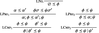
The empty log
tells us nothing about the past, and hence
we have that
 for every log as
expressed by Rule
for every log as
expressed by Rule
 . Rule
 can be
understood as follows: if we have two logs
and
can be
understood as follows: if we have two logs
and
 , then in order to prove that
 holds, we need to prove that both
and
holds, we need to prove that both
and
 hold. Note that here we are using
 and
and
 to denote the application of the
(possibly empty) closing substitutions and to logs
and respectively and that this is needed as
only applies to closed logs.
Rule
to denote the application of the
(possibly empty) closing substitutions and to logs
and respectively and that this is needed as
only applies to closed logs.
Rule
 simply says that if
, then
adding an action at the beginning of will only add more
information to it, and hence,
simply says that if
, then
adding an action at the beginning of will only add more
information to it, and hence,
 holds too. Rule
 says that
 holds if it
is the case that both
and
holds if it
is the case that both
and
 hold.
The definition of
implies that we are taking a
nonlinear interpretation of logs, that is we allow and
hold.
The definition of
implies that we are taking a
nonlinear interpretation of logs, that is we allow and  in
in
 to reference the same actions, in effect duplicating
the information conveyed about the past. This interpretation is
required as the calculus allows the copying of values and their
provenance. Rule
to reference the same actions, in effect duplicating
the information conveyed about the past. This interpretation is
required as the calculus allows the copying of values and their
provenance. Rule
 says that in order to show that
 , we need to show that
holds.
, we need to show that
holds.
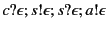
To illustrate the application of the above rules, let us consider the
two logs
 and
and
 . Log
tells us that sent on some unknown channel which it received
on channel while tells us that sent on channel
which it received on channel . Clearly tells us more
information about the past than and the unknown channel in
is actually channel (inferred from ). To show this
using the inference rules above, we first apply Rule
as follows:
. Log
tells us that sent on some unknown channel which it received
on channel while tells us that sent on channel
which it received on channel . Clearly tells us more
information about the past than and the unknown channel in
is actually channel (inferred from ). To show this
using the inference rules above, we first apply Rule
as follows:
Then, we show that
 and
that
and
that
 . The former holds
since
. The former holds
since
 whereas the
latter may be shown to hold by further application of
and
.
whereas the
latter may be shown to hold by further application of
and
.
Proposition 1
The relation
is a partial order.
We interpret the provenance in an annotated value
to be a set of assertions about the past of the value
. These assertions tell us about events that took place in the
system and that are relevant to the value . For example, consider
the value
 , its
provenance tells us that
, its
provenance tells us that
![\begin{inparaenum}[\itshape\upshape (a\upshape )]
\item $v$ was most recently r...
...''$ tells us about the past
of $v$ before it was sent by $b$
\end{inparaenum}](img192.png)
.
It is important here to note that the provenance of does not reveal
the identities of the channels used for communication, nor does it tell
us about the ordering between events in and those in
 or between events in
  and those
in
and those
in  .
.
Assertions such as those above may be encoded in a ``condensed form'' as
logs. We define the function
which maps
 to a log that represents what the provenance
sequence tells us about the past of
to a log that represents what the provenance
sequence tells us about the past of  . The definition of
in Definition 2 below uses a
different grammar for provenance sequences than that given in
Table 1 in order to make the definition of
simpler. It is easy to check, however, that for our
purposes the two grammars are equivalent.
. The definition of
in Definition 2 below uses a
different grammar for provenance sequences than that given in
Table 1 in order to make the definition of
simpler. It is easy to check, however, that for our
purposes the two grammars are equivalent.
Definition 2 (Denotation of provenance)
The function

is
defined inductively on the structure of provenance sequences as follow:
The empty provenance sequence in an
annotated value
 tells us that originated here,
and hence
tells us that originated here,
and hence
 is taken to be the empty log
. The annotated values
is taken to be the empty log
. The annotated values
 and
and
 denote
that was sent (respectively received) on some unknown channel ,
and that before that the logs denoted by
denote
that was sent (respectively received) on some unknown channel ,
and that before that the logs denoted by
 and
and
 occurred in some unknown order. It
is clear that a log
is a partial record
of what took place in a system. Indeed, it does not contain information
about the identities of the channels used for communication, and it
lacks information about the order in which some actions took place. This
is to be expected of course as the provenance of a value is meant to
only record information about actions that are relevant to the value
itself.
occurred in some unknown order. It
is clear that a log
is a partial record
of what took place in a system. Indeed, it does not contain information
about the identities of the channels used for communication, and it
lacks information about the order in which some actions took place. This
is to be expected of course as the provenance of a value is meant to
only record information about actions that are relevant to the value
itself.
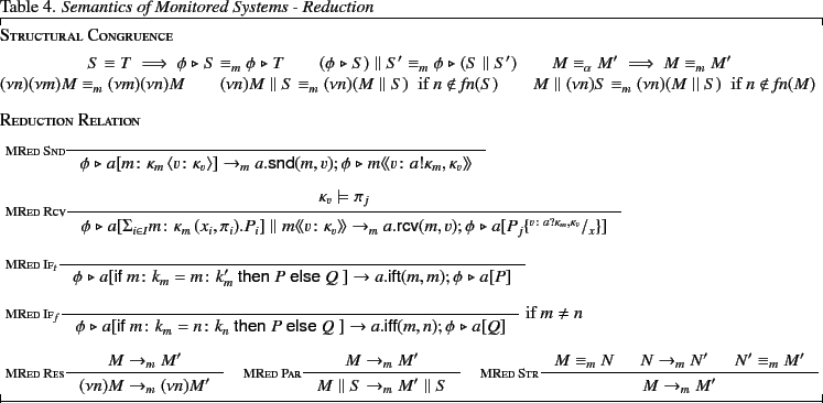
In order to be able to assess the correctness and completeness of
provenance, we introduce the notion of monitored systems. A
monitored system is one where every action that takes place is recorded
in a global log. The global log provides a repository where every
action is logged and whose content is not accessible by principals. It
is only meant as a proof tool against which the properties of provenance
can be formulated and judged.
We use
 to range over monitored systems and give their
formal syntax below.
to range over monitored systems and give their
formal syntax below.
The notation
 denotes the monitored system composed of
global log and system
denotes the monitored system composed of
global log and system  . Restriction
  and parallel
composition
and parallel
composition
 are needed to allow the global log to behave
like other parts of the system with respect to scope extrusion and
intrusion. More specifically, the form allows channel scopes
to be extruded to include the log while the form
is
needed to allow channels whose scope includes the log but not some part
of the system . Note that indeed the above syntax allows exactly one
global log per monitored system. We also define versions of structural
congruence and reduction for monitored systems and denote them by
are needed to allow the global log to behave
like other parts of the system with respect to scope extrusion and
intrusion. More specifically, the form allows channel scopes
to be extruded to include the log while the form
is
needed to allow channels whose scope includes the log but not some part
of the system . Note that indeed the above syntax allows exactly one
global log per monitored system. We also define versions of structural
congruence and reduction for monitored systems and denote them by
 and
and
 respectively. These are given in
Table 4. It should clear from the definition of
that the original provenance tracking semantics of systems is
preserved, and that all
adds is the recording of actions in
the global log. We formalise this in Proposition 2.
This latter makes use of the log erasure function,
respectively. These are given in
Table 4. It should clear from the definition of
that the original provenance tracking semantics of systems is
preserved, and that all
adds is the recording of actions in
the global log. We formalise this in Proposition 2.
This latter makes use of the log erasure function,
 ,
which given a monitored system, removes the log and returns just the
system part of it. The function
is defined inductively on
the structure of monitored systems as follows.
,
which given a monitored system, removes the log and returns just the
system part of it. The function
is defined inductively on
the structure of monitored systems as follows.
Proposition 2
 implies that
 . Vice
versa,
. Vice
versa,
 implies that
for some
implies that
for some
 such that
 .
.
3.4 Correctness
The first provenance property we look at is correctness. A provenance
sequence in an annotated value
is considered
correct if what it tells us about the past of agrees with what
actually took place. This is defined relative to the global log which
is assumed to be a correct and complete record of the past of a system.
If every value in a system has correct provenance, then we say that the
system as a whole has correct provenance. Theorem 1
states that provenance correctness is preserved by the reduction
relation. That is, starting from a system with correct provenance, we
are guaranteed to get a system with correct provenance after reduction.
Definition 3 makes use of two auxiliary functions:
 , which returns the global log of a monitored system, and
 , which returns the set of ``annotated values'' of a monitored
system. The definition of
, by induction on the structure of
monitored systems, is straightforward and hence omitted. This is mostly
the case for
too and hence, we only discuss the most
interesting cases below. The set of values in a monitored system is
defined to be that in its system part (i.e., we ignore the global log and
top level restrictions). This is expressed by the following
three rules:
, which returns the set of ``annotated values'' of a monitored
system. The definition of
, by induction on the structure of
monitored systems, is straightforward and hence omitted. This is mostly
the case for
too and hence, we only discuss the most
interesting cases below. The set of values in a monitored system is
defined to be that in its system part (i.e., we ignore the global log and
top level restrictions). This is expressed by the following
three rules:
For systems, we proceed simply by gathering annotated values, that is
``subterms'' of the form
, and substituting
for any restricted channel names. So for example, we have that
![$ \mathit{values}(a[P]) \triangleq \mathit{values}(P)$](img231.png) ,
,
 ,
,
 , and
, and
 . Note that
restriction here is treated differently from that at the top
level of monitored systems. The rationale behind this discrepancy is
that restricted names at the top level are known to the global log
whereas those occurring here are not. The substitution is done to avoid
any clashes with names appearing in the log and is inspired by
[17]. Definition of
. Note that
restriction here is treated differently from that at the top
level of monitored systems. The rationale behind this discrepancy is
that restricted names at the top level are known to the global log
whereas those occurring here are not. The substitution is done to avoid
any clashes with names appearing in the log and is inspired by
[17]. Definition of
 for processes
is similar.
for processes
is similar.
Definition 3
A monitored system
 has correct provenance
 if for all
in

, we have that
.
Lemma 1
has correct provenance and
 implies that has
correct provenance.
implies that has
correct provenance.
Proof.
We assume that
has correct provenance and that
. We
show that
has correct provenance by induction on the derivation of
. The details of the proof are straightforward and
therefore omitted.

3.5 Towards a Notion of Completeness
We have already shown informally that the provenance of a value is not a
complete record of what took place in the whole system. We formalise
this below.
Definition 4
A monitored system
has complete provenance if for all
in
, we have that
.
Proof.
Let us consider the monitored system
defined as follows:
Assuming
has complete provenance, then it is clear that
has
too. Now, we have that
where
is defined as follows:
does not have complete provenance, since

does
not.
Completeness is too strong since we are requiring every value to have
complete information about the past of the whole system.
In fact, in general it is not even possible for a single value, as it can
be easily demonstrated by considering a system where a value gets
forgotten at some point in the evolution of the system, such as the
following:
where, assuming that does not contain copies of
 , the system will evolve to a state where
is completely forgotten.
, the system will evolve to a state where
is completely forgotten.
4 Related Work
Provenance has been studied in a variety of settings, most prominently
in databases and scientific computing. A major theme of provenance
research in the database community has been that of identifying parts of
the input of a query relevant to parts of its output. The
definition of the provenance notion (i.e., what ``relevant'' means) as
well as the granularity at which data is considered (i.e., what ``parts''
of the input or output constitute) varies depending on the intended
application.
One of the earliest works that studied provenance for database
management systems was by Wang and Madnick in their Polygen model
[24], which aimed to resolve provenance issues for data
composed from multiple sources. Woodruff and Stonebraker
[25] studied a notion of provenance called
lineage. Their aim was to provide fine-grained lineage
information, which they argued was prohibitively expensive to achieve
using metadata. Their approach instead relied on a small amount of
information about the database operations performed and the analysis of
base data. Buneman et al. [5] studied provenance in
the setting of a data model that generalises both relational as well
hierarchical databases. They proposed two different notions of
provenance, which they termed ``why'' and ``where'' provenance, and gave
algorithms to compute the two types of provenance information.
Motivated by the need for formal foundations of provenance, Cheney et
al. [7] proposed a semantic characterisation of
provenance based on dependency analysis. They showed that minimal
dependency provenance is not computable and provided dynamic and static
techniques to approximate it. Green et al. [11]
introduced a model based on semiring valued annotations and showed that
this model generalises several models of annotated relations including
why provenance.
There is a big incentive to support provenance in scientific computing
settings. This stems from the need to allow scientists to understand,
analyse and replicate results of experiments. Some of the projects aimed
at developing middleware to support provenance in this setting include
Chimera [9] (physics and astronomy),
 Grid [23] (biology), CMCS
[21] (chemical sciences), and ESSW
[10] (earth sciences). Bose and Frew [2]
and Simmhan et al. [22] give surveys of the most
important research efforts in this area.
Grid [23] (biology), CMCS
[21] (chemical sciences), and ESSW
[10] (earth sciences). Bose and Frew [2]
and Simmhan et al. [22] give surveys of the most
important research efforts in this area.
5 Conclusion and Future Work
We presented a calculus for provenance in distributed systems. The
semantics of the calculus tracks the provenance of values dynamically
and allows principals to perform tests against it. These tests let
principals decide what data to consume and what to do with it based on
its provenance. We also discussed the semantics of provenance and
studied some of its properties.
We proposed a characterisation of provenance correctness and
completeness based on the notions of monitored systems and global logs.
We showed that based on this characterisation, our provenance is correct
but incomplete. However, as we have mentioned, completeness is too
strong since we are requiring the provenance of every value to be a
complete record of everything that has taken place within the system.
Instead of asking for the provenance to be complete, what is needed is for
provenance to be adequate. What we mean by this is that the
provenance information recorded has to be enough for its intended
application. In developing such an idea, we are interested in using
information about the role each principal played in getting a piece of
data to its current form (and the implied trust relations between
principals), as a measure of how trustworthy a piece of data is likely
to be. Hence, we only need to know about actions that are relevant to
the value at hand, and we only need to know about the principals
involved in the action. We are working on formalising adequacy at the
moment. We also plan to investigate other ways of characterising
provenance properties, for example, based on logic.
Provenance tracking is performed dynamically at the moment as part of
the reduction relation. Although this yields accurate provenance
information, it results in runtime overhead as provenance is computed,
updated and tests are performed against it. We are working on a static
analysis that would alleviate the need for dynamic provenance tracking.
The idea behind it is to analyse the flow of data between principals and
make sure that principals would only receive data with provenance that
matches their expectations.
To keep the calculus simple, we only allowed statically defined patterns
with no binding variables. This means that principals cannot use dynamic
information for their provenance tests nor can they extract part (or
all) of the provenance sequence and use it as data. This is one of the
first extensions we aim to make to the calculus. In addition to this,
provenance is currently tracked by the runtime environment, and
principals are only given ``read-only'' access to it. Moreover, every
principal is able to see the entire provenance sequence, regardless of
the privacy and security policies of other principals. However, in many
applications, principals may wish to control the disclosure of
provenance information about them. We are working on extending the
calculus with such features at the moment. We are also investigating how
to extend the calculus to allow the communication of data structures.
With this, we aim to provide support for scenarios where data is not
only copied and communicated, but also broken down into pieces, combined
with other data, and generally transformed to produce new data. In these
scenarios, the ways in which we may manipulate data usually depend on
its provenance and vice versa. This means that a transformation  of
values and needs to take into account their provenances
of
values and needs to take into account their provenances
 and
and  as well. That is, the result of the
transformation should be of the form
as well. That is, the result of the
transformation should be of the form
 as opposed to
 . The same holds for transformations
 that manipulate the provenance. To be able to express this, we
aim to extend the calculus, along similar lines as the applied
-calculus [1], with data structures and operations
on them.
that manipulate the provenance. To be able to express this, we
aim to extend the calculus, along similar lines as the applied
-calculus [1], with data structures and operations
on them.
- 1
-
ABADI, M., AND FOURNET, C.
Mobile values, new names, and secure communication.
ACM SIGPLAN Notices 36, 3 (Mar. 2001), 104-115.
- 2
-
BOSE, R., AND FREW, J.
Lineage retrieval for scientific data processing: a survey.
ACM Computing Surveys 37, 1 (Mar. 2005), 1-28.
- 3
-
BOUDOL, G.
Asynchrony and the -calculus.
Tech. Rep. 1702, INRIA, Sophia-Antipolis, 1992.
- 4
-
BUNEMAN, P., CHENEY, J., AND VANSUMMEREN, S.
On the expressiveness of implicit provenance in query and update
languages.
In ICDT (2007), vol. 4353 of LNCS, Springer,
pp. 209-223.
- 5
-
BUNEMAN, P., KHANNA, S., AND TAN, W. C.
Why and where: A characterization of data provenance.
In ICDT (2001), vol. 1973 of LNCS, Springer,
pp. 316-330.
- 6
-
CASTAGNA, G., NICOLA, R. D., AND VARACCA, D.
Semantic subtyping for the pi-calculus.
Theoretical Computer Science 398, 1-3 (2008), 217-242.
- 7
-
CHENEY, J., AHMED, A., AND ACAR, U. A.
Provenance as dependency analysis.
In Database Programming Languages (2007), vol. 4797 of LNCS, Springer, pp. 138-152.
- 8
-
CUI, Y., AND WIDOM, J.
Practical lineage tracing in data warehouses.
In ICDE (Mar. 2000), IEEE Computer Society, pp. 367-378.
- 9
-
FOSTER, I. T., VÖCKLER, J.-S., WILDE, M., AND ZHAO, Y.
Chimera: A virtual data system for representing, querying, and
automating data derivation.
In Statistical and Scientific Database Management (2002),
IEEE Computer Society, pp. 37-46.
- 10
-
FREW, J., AND BOSE, R.
Earth system science workbench: A data management infrastructure
for earth science products.
In Statistical and Scientific Database Management (2001),
IEEE Computer Society, pp. 180-189.
- 11
-
GREEN, T. J., KARVOUNARAKIS, G., AND TANNEN, V.
Provenance semirings.
In PODS (2007), ACM, pp. 31-40.
- 12
-
GREENWOOD, M., GOBLE, C., STEVENS, R., ZHAO, J., ADDIS, M., MARVIN, D.,
MOREAU, L., AND OINN, T.
Provenance of e-science experiments - experience from bioinformatics.
Proceedings of the UK OST e-Science Second All Hands Meeting, Jan.
2003.
- 13
-
GROTH, P., MUNROE, S., MILES, S., AND MOREAU, L.
In Lucio Grandinetti (ed.), HPC and Grids in Action.
IOS Press, Jan. 2008, ch. Applying the Provenance Data Model to a
Bioinformatics Case.
- 14
-
HENNESSY, M., AND RIELY, J.
Resource access control in systems of mobile agents.
Information and Computation 173, 1 (Feb 2002), 82-120.
- 15
-
HONDA, K., AND TOKORO, M.
An object calculus for asynchronous communication.
In ECOOP (1991), Springer-Verlag, pp. 133-147.
- 16
-
HOSOYA, H., AND PIERCE, B. C.
Regular expression pattern matching.
In POPL (2001).
Full version in Journal of Functional Programming, 13(6), Nov.
2003, pp. 961-1004.
- 17
-
LHOUSSAINE, C., AND SASSONE, V.
A dependently typed ambient calculus.
In ESOP (2004), vol. 2986 of LNCS, Springer,
pp. 171-187.
- 18
-
MILNER, R.
Communicating and Mobile Systems: The -calculus.
Cambridge University Press, 1999.
- 19
-
MOREAU, L., GROTH, P., MILES, S., VAZQUEZ, J., IBBOTSON, J., JIANG, S.,
MUNROE, S., RANA, O., SCHREIBER, A., TAN, V., AND VARGA, L.
The Provenance of Electronic Data.
Communications of the ACM (Apr. 2008).
- 20
-
MUNISWAMY-REDDY, K.-K., HOLLAND, D. A., BRAUN, U., AND SELTZER, M. I.
Provenance-aware storage systems.
In USENIX Annual Technical Conference, General Track (2006),
USENIX, pp. 43-56.
- 21
-
PANCERELLA, C., MYERS, J., AND RAHN, L.
Data provenance in the collaboratory for multiscale chemical science
(CMCS).
Workshop on Data Derivation and Provenance (Jan 2002).
- 22
-
SIMMHAN, Y. L., PLALE, B., AND GANNON, D.
A survey of data provenance in e-science.
SIGMOD Record 34, 3 (2005), 31-36.
- 23
-
STEVENS, R. D., ROBINSON, A. J., AND GOBLE, C. A.
myGrid: personalised bioinformatics on the information grid.
In ISMB (Supplement of Bioinformatics) (2003), pp. 302-304.
- 24
-
WANG, Y. R., AND MADNICK, S. E.
A polygen model for heterogeneous database systems: The source
tagging perspective.
In VLDB (1990), Morgan Kaufmann Publishers Inc.,
pp. 519-538.
- 25
-
WOODRUFF, A., AND STONEBRAKER, M.
Supporting fine-grained data lineage in a database visualization
environment.
In Proceedings of the Thirteenth International Conference on
Data Engineering (1997), IEEE Computer Society, pp. 91-102.
A Formal Model of Provenance in Distributed Systems
This document was generated using the
LaTeX2HTML translator Version 2002-2-1 (1.71)
Copyright © 1993, 1994, 1995, 1996,
Nikos Drakos,
Computer Based Learning Unit, University of Leeds.
Copyright © 1997, 1998, 1999,
Ross Moore,
Mathematics Department, Macquarie University, Sydney.
The command line arguments were:
latex2html -split 0 -show_section_numbers -local_icons -no_navigation sfs_html
The translation was initiated by Issam on 2009-02-12
Footnotes
- ...
computation.1
- In a typical implementation of our language, we
would assign the provenance tracking tier to a trusted underlying
middleware.
- ... ignored.2
- Depending on the intended
application, the provenance of the two values tested could be useful and
hence should be tracked in the continuation. This is not considered
here however as it is not important for the aims of this paper.
Issam
2009-02-12