OSDI '06 Paper
Pp. 205–218 of the Proceedings
Bigtable: A Distributed Storage System for Structured Data
Fay Chang, Jeffrey Dean, Sanjay Ghemawat, Wilson C. Hsieh, Deborah A. Wallach
Mike Burrows, Tushar Chandra, Andrew Fikes, Robert E. Gruber
{fay,jeff,sanjay,wilsonh,kerr,m3b,tushar,fikes,gruber}@google.com
Google, Inc.
Abstract:
Bigtable is a distributed storage system for managing structured data
that is designed to scale to a very large size:
petabytes of data across thousands of commodity servers. Many
projects at Google store data in Bigtable, including web indexing,
Google Earth, and Google Finance. These applications place very
different demands on Bigtable, both in terms of data size (from URLs
to web pages to satellite imagery) and latency requirements (from
backend bulk processing to real-time data serving). Despite these
varied demands, Bigtable has successfully provided a flexible,
high-performance solution for all of these Google products. In this
paper we describe the simple data model provided by Bigtable, which
gives clients dynamic control over data layout and format, and we
describe the design and implementation of Bigtable.
Over the last two and a half years we have designed, implemented, and
deployed a distributed storage system for managing structured data at
Google called Bigtable. Bigtable is designed to reliably scale to
petabytes of data and thousands of machines. Bigtable has achieved
several goals: wide applicability, scalability, high performance, and
high availability. Bigtable is used by more than sixty Google
products and projects, including Google Analytics, Google Finance, Orkut,
Personalized Search, Writely, and Google Earth.
These products use Bigtable for a variety of
demanding workloads, which range from throughput-oriented
batch-processing jobs to latency-sensitive serving of data to end
users. The Bigtable clusters
used by these products span a wide range of configurations, from a
handful to thousands of servers, and store up to several hundred
terabytes of data.
In many ways, Bigtable resembles a database: it shares many
implementation strategies with databases. Parallel
databases [14] and main-memory databases [13]
have achieved scalability and high performance, but Bigtable provides
a different interface than such systems. Bigtable does not support a
full relational data model; instead, it provides clients with a simple
data model that supports dynamic control over data layout and format,
and allows clients to reason about the locality properties of the data
represented in the underlying storage. Data is indexed using
row and column names that can be arbitrary strings. Bigtable
also treats data as uninterpreted strings, although clients often
serialize various forms of structured and semi-structured data into
these strings. Clients can control the locality of their data through
careful choices in their schemas. Finally, Bigtable schema parameters
let clients dynamically control whether to serve data out of memory or
from disk.
Section 2 describes the data model in more detail,
and Section 3 provides an overview of the client API.
Section 4 briefly describes the underlying
Google infrastructure on which Bigtable depends.
Section 5 describes the fundamentals of the
Bigtable implementation, and Section 6
describes some of the refinements that we made to improve Bigtable's
performance. Section 7 provides measurements
of Bigtable's performance. We describe several examples of how
Bigtable is used at Google in Section 8, and discuss
some lessons we learned in designing and supporting Bigtable in
Section 9. Finally, Section 10
describes related work, and Section 11 presents
our conclusions.
2 Data Model
A Bigtable is a sparse, distributed, persistent multi-dimensional sorted map.
The map is indexed by a row key, column key, and a timestamp;
each value in the map is an uninterpreted array of bytes.
We settled on this data model after examining a variety of potential
uses of a Bigtable-like system. As one concrete example that drove
some of our design decisions, suppose we want to keep a copy of a large
collection of web pages and related information that could be used by
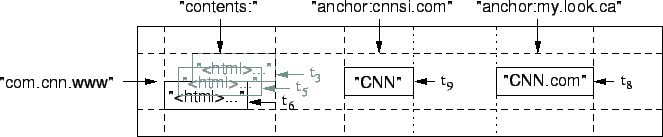
many different projects; let us call this particular table the Webtable. In Webtable, we would use URLs as row keys, various
aspects of web pages as column names, and store the contents of the
web pages in the contents: column under the timestamps when
they were fetched, as illustrated in Figure 1.
Figure 1: A slice of an example table that stores Web pages.
The row name is a reversed URL. The contents column family
contains the page contents, and the anchor column family
contains the text of any anchors that reference the page. CNN's
home page is referenced by both the Sports Illustrated and the
MY-look home pages, so the row contains columns named
anchor:cnnsi.com and anchor:my.look.ca. Each
anchor cell has one version; the contents column has three versions,
at timestamps  , ,  , and , and  . .
|
The row keys in a table are arbitrary strings (currently up to 64KB in
size, although 10-100 bytes is a typical size for most of our users).
Every read or write of data under a single row key is atomic
(regardless of the number of different columns being read or written
in the row), a design decision that makes it easier for clients to
reason about the system's behavior in the presence of concurrent
updates to the same row.
Bigtable maintains data in lexicographic order by row key. The row
range for a table is dynamically partitioned. Each row range is
called a tablet, which is the unit of distribution and load
balancing. As a result, reads of short row ranges are efficient and
typically require communication with only a small number of machines.
Clients can exploit this property by selecting their row keys so that
they get good locality for their data accesses. For example, in
Webtable, pages in the same domain are grouped together into
contiguous rows by reversing the hostname components of the URLs. For
example, we store data for maps.google.com/index.html under
the key com.google.maps/index.html. Storing pages from the
same domain near each other makes some host and domain analyses more
efficient.
Column keys are grouped into sets called column families, which
form the basic unit of access control. All data stored in a column
family is usually of the same type (we compress data in the same
column family together). A column family must be created before data
can be stored under any column key in that family; after a family has
been created, any column key within the family can be used. It is
our intent that the number of distinct column families in a table be
small (in the hundreds at most), and that families rarely change
during operation. In contrast, a table may have an unbounded number
of columns.
A column key is named using the following syntax: family:qualifier. Column family names must be printable, but qualifiers
may be arbitrary strings. An example column family for the Webtable
is language, which stores the language in which a web page
was written. We use only one column key in the language
family, and it stores each web page's language ID. Another useful
column family for this table is anchor; each column key in this
family represents a single anchor, as shown in
Figure 1. The qualifier is the name of the
referring site; the cell contents is the link text.
Access control and both disk and memory accounting are performed at
the column-family level. In our Webtable example, these controls
allow us to manage several different types of applications: some that
add new base data, some that read the base data and create derived
column families, and some that are only allowed to view existing data
(and possibly not even to view all of the existing families for
privacy reasons).
Each cell in a Bigtable can contain multiple versions of the same
data; these versions are indexed by timestamp. Bigtable timestamps
are 64-bit integers. They can be assigned by Bigtable, in which case
they represent "real time" in microseconds, or be explicitly
assigned by client applications. Applications that need to
avoid collisions must generate unique timestamps themselves.
Different versions of a cell are stored in decreasing timestamp order,
so that the most recent versions can be read first.
To make the management of versioned data less onerous, we support two
per-column-family settings that tell Bigtable to garbage-collect cell
versions automatically. The client can specify either that only the
last n versions of a cell be kept, or that only new-enough
versions be kept (e.g., only keep values that were written in the last
seven days).
In our Webtable example, we set the timestamps of the crawled pages
stored in the contents: column to the times at which these
page versions were actually crawled. The garbage-collection mechanism
described above lets us keep only the most recent three versions of
every page.
3 API
The Bigtable API provides functions for creating
and deleting tables and column families. It also provides functions
for changing cluster, table, and column family metadata, such as
access control rights.
Client applications can write or delete values in Bigtable, look up
values from individual rows, or iterate over a subset of the data
in a table. Figure 2 shows C++ code that
uses a RowMutation abstraction to perform a series of updates.
(Irrelevant details were elided to keep the example short.)
The call to Apply performs an atomic mutation to the
Webtable: it adds one anchor to www.cnn.com and deletes a
different anchor.
Figure 2:
Writing to Bigtable.
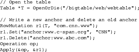 |
Figure 3 shows C++ code that uses a Scanner abstraction to iterate over all anchors in a particular row.
Figure 3:
Reading from Bigtable.
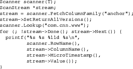 |
Clients can iterate over multiple column families, and there are several
mechanisms for limiting the rows, columns, and timestamps produced by a scan.
For example, we could restrict the scan above to only produce anchors whose columns
match the regular expression anchor:*.cnn.com,
or to only produce anchors whose timestamps fall within ten days of the current time.
Bigtable supports several other features that allow the user to
manipulate data in more complex ways. First, Bigtable supports
single-row transactions, which can be used to perform atomic
read-modify-write sequences on data stored under a single row key.
Bigtable does not currently support general transactions across row
keys, although it provides an interface for batching writes across
row keys at the clients. Second, Bigtable allows cells to be
used as integer counters. Finally, Bigtable supports the execution of
client-supplied scripts in the address spaces of the servers. The
scripts are written in a language developed at Google for processing
data called Sawzall [28]. At the moment, our Sawzall-based
API does not allow client scripts to write back into Bigtable, but it
does allow various forms of data transformation, filtering based on
arbitrary expressions, and summarization via a variety of operators.
Bigtable can be used with MapReduce [12], a framework for
running large-scale parallel computations developed at Google. We
have written a set of wrappers that allow a Bigtable to be used
both as an input source and as an output target for MapReduce jobs.
4 Building Blocks
Bigtable is built on several other pieces of Google infrastructure.
Bigtable uses the distributed Google File System
(GFS) [17] to store log and data files. A Bigtable
cluster typically operates in a shared pool of machines that run a
wide variety of other distributed applications, and Bigtable processes
often share the same machines with processes from other applications.
Bigtable depends on a cluster management system for scheduling jobs,
managing resources on shared machines, dealing with machine failures,
and monitoring machine status.
The Google SSTable file format is used internally to store
Bigtable data. An SSTable provides a persistent, ordered immutable
map from keys to values, where both keys and values are arbitrary byte
strings. Operations are provided to look up the value associated with
a specified key, and to iterate over all key/value pairs in a
specified key range. Internally, each SSTable contains a sequence
of blocks (typically each block is 64KB in size, but this is
configurable). A block index (stored at the end of the SSTable) is
used to locate blocks; the index is loaded into memory when the
SSTable is opened. A lookup can be performed with a single disk
seek: we first find the appropriate block by performing a binary
search in the in-memory index, and then reading the appropriate block
from disk. Optionally, an SSTable can be completely mapped into
memory, which allows us to perform lookups and scans without touching
disk.
Bigtable relies on a highly-available and persistent distributed lock
service called Chubby [8]. A Chubby service consists of
five active replicas, one of which is elected to be the master and
actively serve requests. The service is live when a majority of
the replicas are running and can communicate with each other. Chubby
uses the Paxos algorithm [9,23] to keep its replicas
consistent in the face of failure. Chubby provides a namespace that
consists of directories and small files. Each directory or file can
be used as a lock, and reads and writes to a file are atomic. The
Chubby client library provides consistent caching of Chubby files.
Each Chubby client maintains a session with a Chubby service.
A client's session expires if it is unable to renew its session lease
within the lease expiration time. When a client's session expires, it
loses any locks and open handles. Chubby clients can also register
callbacks on Chubby files and directories for notification of changes
or session expiration.
Bigtable uses Chubby for a variety of tasks: to ensure that there is
at most one active master at any time; to store the bootstrap location
of Bigtable data (see Section 5.1); to
discover tablet servers and finalize tablet server deaths (see
Section 5.2); to store Bigtable schema
information (the column family information for each table);
and to store access control lists. If Chubby becomes unavailable for
an extended period of time, Bigtable becomes unavailable.
We recently measured this effect in 14 Bigtable clusters spanning 11 Chubby
instances. The average percentage of Bigtable server hours during which some
data stored in Bigtable was not available due to Chubby unavailability (caused
by either Chubby outages or network issues) was 0.0047%. The percentage for
the single cluster that was most affected by Chubby unavailability was
0.0326%.
5 Implementation
The Bigtable implementation has three major components: a library that
is linked into every client, one master server, and many tablet
servers. Tablet servers can be dynamically added (or removed) from a
cluster to accomodate changes in workloads.
The master is responsible for assigning tablets to tablet servers,
detecting the addition and expiration of tablet servers, balancing
tablet-server load, and garbage collection of files in GFS. In
addition, it handles schema changes such as table and column family
creations.
Each tablet server manages a set of tablets (typically we have
somewhere between ten to a thousand tablets per tablet server). The
tablet server handles read and write requests to the tablets that it
has loaded, and also splits tablets that have grown too
large.
As with many single-master distributed storage
systems [17,21], client data does not move through
the master: clients communicate directly with tablet servers for reads
and writes. Because Bigtable clients do not rely on the master for
tablet location information, most clients never communicate with
the master. As a result, the master is lightly loaded in practice.
A Bigtable cluster stores a number of tables. Each table consists of
a set of tablets, and each tablet contains all data associated with a
row range. Initially, each table consists of just one tablet. As a
table grows, it is automatically split into multiple tablets, each
approximately 100-200 MB in size by default.
5.1 Tablet Location
We use a three-level hierarchy analogous to that of a
B+-tree [10] to store tablet location information
(Figure 4).
Figure 4:
Tablet location hierarchy.
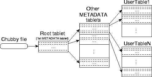 |
The first level is a file stored in Chubby that contains the location
of the root tablet. The root tablet contains the location
of all tablets in a special METADATA table. Each METADATA tablet
contains the location of a set of user tablets. The root
tablet is just the first tablet in the METADATA table, but is
treated specially—it is never split—to ensure that the tablet
location hierarchy has no more than three levels.
The METADATA table stores the location of a tablet under a row key
that is an encoding of the tablet's table identifier and its end row.
Each METADATA row stores approximately 1KB of data in memory. With a
modest limit of 128 MB METADATA tablets, our three-level location
scheme is sufficient to address  tablets (or tablets (or  bytes
in 128 MB tablets). bytes
in 128 MB tablets).
The client library caches tablet locations. If the client does not
know the location of a tablet, or if it discovers that cached location
information is incorrect, then it recursively moves up the tablet
location hierarchy. If the client's cache is empty, the location
algorithm requires three network round-trips, including one read from
Chubby. If the client's cache is stale, the location algorithm could
take up to six round-trips, because stale cache entries are only
discovered upon misses (assuming that METADATA tablets do not move
very frequently). Although tablet locations are stored in memory, so
no GFS accesses are required, we further reduce this cost in the
common case by having the client library prefetch tablet locations: it
reads the metadata for more than one tablet whenever it reads the
METADATA table.
We also store secondary information in the METADATA table, including
a log of all events pertaining to each tablet (such as when a server
begins serving it). This information is helpful for
debugging and performance analysis.
5.2 Tablet Assignment
Each tablet is assigned to one tablet server at a time.
The master keeps track of the set of live tablet servers, and the current
assignment of tablets to tablet servers, including which tablets are
unassigned. When a tablet is unassigned, and a tablet server
with sufficient room for the tablet is available, the master assigns the
tablet by sending a tablet load request to the tablet server.
Bigtable uses Chubby to keep track of tablet servers.
When a tablet server starts, it creates, and acquires an exclusive lock on,
a uniquely-named file in a specific Chubby directory. The master monitors
this directory (the servers directory) to discover tablet servers.
A tablet server stops serving its tablets if it loses its exclusive
lock: e.g., due to a network partition that caused the server to lose its
Chubby session. (Chubby provides an efficient mechanism that allows a
tablet server to check whether it still holds its lock without incurring
network traffic.) A tablet server will attempt to reacquire an exclusive lock
on its file as long as the file still exists. If the file no longer exists,
then the tablet server will never be able to serve again, so it kills itself.
Whenever a tablet server terminates (e.g., because the cluster management
system is removing the tablet server's machine from the cluster), it attempts
to release its lock so that the master will reassign its tablets more quickly.
The master is responsible for detecting when a tablet server is no longer
serving its tablets, and for reassigning those tablets as soon as possible.
To detect when a tablet server is no longer serving its tablets, the master
periodically asks each tablet server for the status of its lock.
If a tablet server reports that it has lost its lock, or if the master was
unable to reach a server during its last several attempts, the
master attempts to acquire an exclusive lock on the server's file. If the
master is able to acquire the lock, then Chubby is live and the tablet server
is either dead or having trouble reaching Chubby, so the master ensures that
the tablet server can never serve again by deleting its server file. Once a
server's file has been deleted, the master can move all the tablets that were
previously assigned to that server into the set of unassigned tablets.
To ensure that a Bigtable cluster is not
vulnerable to networking issues between the master and Chubby, the master
kills itself if its Chubby session expires. However, as described above,
master failures do not change the assignment of tablets to tablet servers.
When a master is started by the cluster management system, it needs to
discover the current tablet assignments before it can
change them. The master executes the
following steps at startup. (1) The master grabs a unique master lock in Chubby, which prevents concurrent master instantiations.
(2) The master scans the servers directory in Chubby to find the live
servers. (3) The master communicates with every live tablet
server to discover what tablets are already assigned to each server.
(4) The master scans the METADATA table to learn the set of
tablets. Whenever this scan encounters a tablet that is not already
assigned, the master adds the tablet to the set of unassigned tablets,
which makes the tablet eligible for tablet assignment.
One complication is that the scan of the METADATA table cannot happen
until the METADATA tablets have been assigned. Therefore, before
starting this scan (step 4), the master adds the root tablet to the
set of unassigned tablets if an assignment for the root tablet was not
discovered during step 3. This addition ensures that the
root tablet will be assigned. Because the root tablet contains the
names of all METADATA tablets, the master knows about all of them
after it has scanned the root tablet.
The set of existing tablets only changes when a table is created or
deleted, two existing tablets are merged to form one larger tablet,
or an existing tablet is split into two smaller tablets. The master
is able to keep track of these changes because it initiates all but
the last. Tablet splits are treated specially since they are
initiated by a tablet server. The tablet server commits the split by
recording information for the new tablet in the METADATA table. When
the split has committed, it notifies the master. In case the split
notification is lost (either because the tablet server or the master
died), the master detects the new tablet when it asks a tablet server
to load the tablet that has now split. The tablet server will notify
the master of the split, because the tablet entry it finds in the
METADATA table will specify only a portion of the tablet that the
master asked it to load.
5.3 Tablet Serving
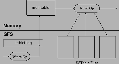
The persistent state of a tablet is stored in GFS, as illustrated in
Figure 5. Updates are committed to a commit log that
stores redo records. Of these updates, the recently committed ones are
stored in memory in a sorted buffer called a memtable; the older
updates are stored in a sequence of SSTables.
Figure 5:
Tablet Representation
 |
To recover a tablet, a tablet server reads its metadata from
the METADATA table. This metadata contains the list of SSTables that comprise a tablet and a set of a redo points, which are pointers
into any commit logs that may contain data for the tablet. The server
reads the indices of the SSTables into memory and reconstructs the
memtable by applying all of the updates that have committed since the
redo points.
When a write operation arrives at a tablet server, the server checks
that it is well-formed, and that the sender is authorized to perform
the mutation. Authorization is performed by reading the list of
permitted writers from a Chubby file (which is almost always a hit
in the Chubby client cache). A valid mutation is written to the commit
log. Group commit is used to improve the throughput of lots of small
mutations [13,16]. After the write has been
committed, its contents are inserted into the memtable.
When a read operation arrives at a tablet server, it is
similarly checked for well-formedness and proper authorization. A
valid read operation is executed on a merged view of the sequence of
SSTables and the memtable. Since the SSTables and the memtable
are lexicographically sorted data structures, the merged view can be
formed efficiently.
Incoming read and write operations can continue while tablets are
split and merged.
As write operations execute, the size of the memtable increases. When
the memtable size reaches a threshold, the memtable is frozen, a new
memtable is created, and the frozen memtable is converted to an
SSTable and written to GFS. This minor compaction process
has two goals: it shrinks the memory usage of the tablet server, and
it reduces the amount of data that has to be read from the commit log
during recovery if this server dies. Incoming read and write
operations can continue while compactions occur.
Every minor compaction creates a new SSTable. If this behavior
continued unchecked, read operations might need to merge updates from
an arbitrary number of SSTables. Instead, we bound the number of such files
by periodically executing a merging compaction in the
background. A merging compaction reads the contents of a few
SSTables and the memtable, and writes out a new SSTable.
The input SSTables and memtable can be discarded as soon
as the compaction has finished.
A merging compaction that rewrites all SSTables into exactly one SSTable is called a major compaction. SSTables produced by non-major
compactions can contain special deletion entries that suppress
deleted data in older SSTables that are still live. A major
compaction, on the other hand, produces an SSTable that contains no
deletion information or deleted data. Bigtable cycles through all of
its tablets and regularly applies major compactions to them.
These major compactions allow Bigtable to reclaim resources used by
deleted data, and also allow it to ensure that deleted data
disappears from the system in a timely fashion, which is important for
services that store sensitive data.
6 Refinements
The implementation described in the previous section required a number of
refinements to achieve the high performance, availability, and reliability
required by our users. This section describes portions of the
implementation in more detail in order to highlight these refinements.
Clients can group multiple column families together into a locality group. A separate SSTable is generated for each locality
group in each tablet. Segregating column families that are not
typically accessed together into separate locality groups enables more
efficient reads. For example, page metadata in Webtable
(such as language and checksums)
can be in one locality group, and the
contents of the page can be in a different group: an
application that wants to read the metadata does not need to
read through all of the page contents.
In addition, some useful tuning parameters can be specified on a
per-locality group basis. For example, a locality group can be
declared to be in-memory. SSTables for in-memory locality groups
are loaded lazily into the memory of the tablet server. Once loaded,
column families that belong to such locality groups can be read
without accessing the disk. This feature is useful for small pieces
of data that are accessed frequently: we use it internally for the
location column family in the METADATA table.
Clients can control whether or not the SSTables for a locality
group are compressed, and if so, which compression format is used.
The user-specified compression format is applied to each SSTable block (whose size is controllable via a locality group
specific tuning parameter). Although we lose some space by
compressing each block separately, we benefit in that small
portions of an SSTable can be read without decompressing the entire
file.
Many clients use a two-pass custom compression scheme.
The first pass uses Bentley and McIlroy's scheme [6],
which compresses long common strings across a large window.
The second pass uses a fast compression algorithm that looks
for repetitions in a small 16 KB window of the data. Both compression
passes are very fast—they encode at 100-200 MB/s, and decode at
400-1000 MB/s on modern machines.
Even though we emphasized speed instead of
space reduction when choosing our compression algorithms, this two-pass
compression scheme does surprisingly well. For example, in Webtable,
we use this compression scheme to store Web page contents. In one
experiment, we stored a large number of documents in a compressed
locality group. For the purposes of the experiment, we limited
ourselves to one version of each document instead of storing all
versions available to us. The scheme achieved a 10-to-1
reduction in space. This is much better than typical Gzip reductions
of 3-to-1 or 4-to-1 on HTML pages because of the way Webtable rows are
laid out: all pages from a single host are stored close to each
other. This allows the Bentley-McIlroy algorithm to identify large
amounts of shared boilerplate in pages from the same host. Many
applications, not just Webtable, choose their row names so that
similar data ends up clustered, and therefore achieve very good
compression ratios. Compression ratios get even better when we store
multiple versions of the same value in Bigtable.
To improve read performance, tablet servers use two levels of caching.
The Scan Cache is a higher-level cache that caches the key-value pairs
returned by the SSTable interface to the tablet server code. The
Block Cache is a lower-level cache that caches SSTables blocks that
were read from GFS. The Scan Cache is most useful for applications
that tend to read the same data repeatedly. The Block Cache is
useful for applications that tend to read data that is close to the
data they recently read (e.g., sequential reads, or random reads of
different columns in the same locality group within a hot row).
As described in Section 5.3, a read operation has to
read from all SSTables that make up the state of a tablet. If these
SSTables are not in memory, we may end up doing many disk accesses.
We reduce the number of accesses by allowing clients to specify that
Bloom filters [7] should be created for SSTables in
a particular locality group. A Bloom filter allows us to ask whether
an SSTable might contain any data for a specified row/column pair.
For certain applications, a small amount of tablet server memory used
for storing Bloom filters drastically reduces the number of disk seeks
required for read operations. Our use of Bloom filters also implies
that most lookups for non-existent rows or columns do not need to
touch disk.
If we kept the commit log for each tablet in a separate log
file, a very large number of files would be
written concurrently in GFS. Depending on the underlying file
system implementation on each GFS server, these writes could cause a large
number of disk seeks to write to the different physical log files. In
addition, having separate log files per tablet also reduces the
effectiveness of the group commit optimization,
since groups would tend to be smaller. To fix these issues, we append
mutations to a single commit log per tablet server, co-mingling mutations
for different tablets in the same physical log file [18,20].
Using one log provides significant performance benefits during normal
operation, but it complicates recovery. When a tablet server dies,
the tablets that it served will be moved to a large
number of other tablet servers: each server typically loads
a small number of the original server's tablets.
To recover the state for a tablet, the new tablet server needs to
reapply the mutations for that tablet from the commit log written by
the original tablet server. However, the mutations for these tablets
were co-mingled in the same physical log file. One approach would be
for each new tablet server to read this full commit log file and
apply just the entries needed for the tablets it needs to recover.
However, under such a scheme, if 100 machines were each assigned
a single tablet from a failed tablet server, then the log file
would be read 100 times (once by each server).
We avoid duplicating log reads by first sorting the commit log entries
in order of the keys
In the sorted
output, all mutations for a particular tablet are contiguous and can
therefore be read efficiently with one disk seek followed by a
sequential read. To parallelize the sorting, we partition the log
file into 64 MB segments, and sort each segment in parallel on
different tablet servers. This sorting process is coordinated by the
master and is initiated when a tablet server indicates that
it needs to recover mutations from some commit log file.
Writing commit logs to GFS sometimes causes performance hiccups for a
variety of reasons (e.g., a GFS server machine involved in the write
crashes, or the network paths traversed to reach the particular set of
three GFS servers is suffering network congestion, or is heavily
loaded). To protect mutations from GFS latency spikes, each tablet
server actually has two log writing threads, each writing to its own
log file; only one of these two threads is actively in use at a time.
If writes to the active log file are performing poorly, the log file
writing is switched to the other thread, and mutations that are in the
commit log queue are written by the newly active log writing thread.
Log entries contain sequence numbers to allow the recovery process to
elide duplicated entries resulting from this log switching process.
If the master moves a tablet from one tablet server to another, the
source tablet server first does a minor compaction on that tablet.
This compaction reduces recovery time by reducing the amount of
uncompacted state in the tablet server's commit log. After finishing
this compaction, the tablet server stops serving the tablet. Before
it actually unloads the tablet, the tablet server does another
(usually very fast) minor compaction to eliminate any remaining
uncompacted state in the tablet server's log that arrived while the
first minor compaction was being performed. After this second minor
compaction is complete, the tablet can be loaded on another tablet
server without requiring any recovery of log entries.
Besides the SSTable caches, various other parts of the Bigtable system
have been simplified by the fact that all of the SSTables that we
generate are immutable. For example, we do not need any
synchronization of accesses to the file system when reading from
SSTables. As a result, concurrency control over rows can be
implemented very efficiently. The only mutable data structure that is
accessed by both reads and writes is the memtable. To reduce
contention during reads of the memtable, we make each memtable row
copy-on-write and allow reads and writes to proceed in parallel.
Since SSTables are immutable, the problem of permanently removing
deleted data is transformed to garbage collecting obsolete SSTables.
Each tablet's SSTables are registered in the METADATA table. The
master removes obsolete SSTables as a mark-and-sweep garbage
collection [25] over the set of SSTables, where the
METADATA table contains the set of roots.
To delete obsolete files in a small Bigtable cluster, the master periodically
gathers the name of all the existing files for its cluster by scanning the
appropriate directory tree, then scans the METADATA table to obtain the
set of all live files for its cluster, and finally deletes any files in
the former but not latter set. (The METADATA table row for a tablet
contains the names of all files storing data for that tablet.) This
process does not scale well, so in a larger Bigtable cluster, the master
splits this process into smaller chunks, so that it only needs to read a
portion of the directory tree and the METADATA table in order to detect
and delete the dead files in that portion of the directory tree.
Finally, the immutability of SSTables enables us to split tablets
quickly. Instead of generating a new set of SSTables for each child
tablet, we let the child tablets share the SSTables of the parent
tablet.
7 Performance Evaluation
We set up a Bigtable cluster with N tablet servers to measure the
performance and scalability of Bigtable as N is varied. The tablet
servers were configured to use 1 GB of memory and to write to a GFS
cell consisting of 1786 machines with two 400 GB IDE hard drives each.
N client machines generated the Bigtable load used for these
tests. (We used the same number of clients as tablet servers
to ensure that clients were never a bottleneck.) Each machine
had two dual-core Opteron 2 GHz chips, enough physical memory to
hold the working set of all running processes,
and a single gigabit Ethernet link. The machines were
arranged in a two-level tree-shaped switched network with
approximately 100-200 Gbps of aggregate bandwidth available at the
root. All of the machines were in the same hosting facility and
therefore the round-trip time between any pair of machines was less than
a millisecond.
The tablet servers and master, test clients, and GFS servers all ran
on the same set of machines. Every machine ran a GFS
server. Some of the machines also ran either a tablet server, or
a client process, or processes from other jobs that were using the
pool at the same time as these experiments.
R is the distinct number of Bigtable row keys involved in the test. R
was chosen so that each benchmark read or wrote approximately 1 GB of
data per tablet server.
The sequential write benchmark used row keys with names 0 to R-1.
This space of row keys was partitioned into 10N equal-sized
ranges. These ranges were assigned to the N clients by a central
scheduler that assigned the next available range to a client as soon
as the client finished processing the previous range assigned to it.
This dynamic assignment helped mitigate the effects of performance
variations caused by other processes running on the client machines.
We wrote a single string under each row key. Each string was
generated randomly and was therefore uncompressible. In addition,
strings under different row key were distinct, so no cross-row
compression was possible. The random write benchmark was
similar except that the row key was hashed modulo R immediately
before writing so that the write load was spread roughly uniformly
across the entire row space for the entire duration of the benchmark.
The sequential read benchmark generated row keys in exactly
the same way as the sequential write benchmark, but instead of writing
under the row key, it read the string stored under the row key
(which was written by an earlier invocation of the sequential write
benchmark). Similarly, the random read benchmark shadowed the
operation of the random write benchmark.
The scan benchmark is similar to the sequential read
benchmark, but uses support provided by the Bigtable API for scanning
over all values in a row range. Using a scan reduces the number of RPCs
executed by the benchmark since a single RPC fetches a large sequence
of values from a tablet server.
The random reads (mem) benchmark is similar to the random
read benchmark, but the locality group that contains the benchmark
data is marked as in-memory, and therefore the reads are
satisfied from the tablet server's memory instead of requiring a GFS
read. For just this benchmark, we reduced the amount of data per
tablet server from 1 GB to 100 MB so that it would fit comfortably in
the memory available to the tablet server.
Figure 6 shows two views on the performance of
our benchmarks when reading and writing 1000-byte values to Bigtable.
The table shows the number of operations per second per tablet server;
the graph shows the aggregate number of operations per second.
Figure 6:
Number of 1000-byte values read/written per
second. The table shows the rate per tablet server; the graph shows
the aggregate rate.
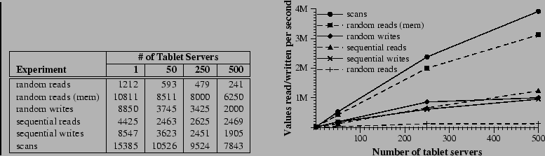 |
Let us first consider performance with just one tablet server. Random
reads are slower than all other operations by an order of magnitude or
more. Each random read involves the transfer of a 64 KB SSTable block over the network from GFS to a tablet server, out of which only
a single 1000-byte value is used. The tablet server executes
approximately 1200 reads per second, which translates into
approximately 75 MB/s of data read from GFS. This bandwidth is enough
to saturate the tablet server CPUs because of overheads in our
networking stack, SSTable parsing, and Bigtable code, and is also
almost enough to saturate the network links used in our system.
Most Bigtable applications with this type of an access
pattern reduce the block size to a smaller value, typically 8KB.
Random reads from memory are much faster since each 1000-byte read is
satisfied from the tablet server's local memory without fetching a
large 64 KB block from GFS.
Random and sequential writes perform better than random reads
since each tablet server appends all incoming writes to a single
commit log and uses group commit to stream these writes efficiently to
GFS. There is no significant difference between the performance of
random writes and sequential writes; in both cases, all writes
to the tablet server are recorded in the same commit log.
Sequential reads perform better than random reads since every 64 KB
SSTable block that is fetched from GFS is stored into our
block cache, where it is used to serve the next 64 read requests.
Scans are even faster since the tablet server can return a large
number of values in response to a single client RPC, and therefore RPC
overhead is amortized over a large number of values.
Aggregate throughput increases dramatically, by over a factor of a
hundred, as we increase the number of tablet servers in the system
from 1 to 500. For example, the performance of random reads from
memory increases by almost a factor of 300 as the number of tablet
server increases by a factor of 500. This behavior occurs because the
bottleneck on performance for this benchmark is the individual tablet
server CPU.
However, performance does not increase linearly. For
most benchmarks, there is a significant drop in
per-server throughput when going from 1 to 50 tablet servers. This drop is
caused by imbalance in load in multiple server configurations, often
due to other processes contending for CPU and network. Our
load balancing algorithm attempts to deal with this imbalance, but
cannot do a perfect job for two main reasons: rebalancing is throttled
to reduce the number of tablet movements (a tablet is unavailable for
a short time, typically less than one second, when it is moved), and
the load generated by our benchmarks shifts around as the benchmark
progresses.
The random read benchmark shows the worst scaling (an increase in
aggregate throughput by only a factor of 100 for a 500-fold increase
in number of servers). This behavior occurs because (as explained above) we
transfer one large 64KB block over the network for every 1000-byte
read. This transfer saturates various shared 1 Gigabit links in our network
and as a result, the per-server throughput drops significantly as we
increase the number of machines.
8 Real Applications
As of August 2006, there are 388 non-test Bigtable clusters running
in various Google machine clusters, with a
combined total of about 24,500 tablet servers.
Table 1 shows a rough distribution of tablet servers per cluster.
Many of these clusters are used for development purposes and
therefore are idle for significant periods. One group of 14 busy
clusters with 8069 total tablet servers saw an aggregate volume of more
than 1.2 million requests per second, with incoming RPC traffic of
about 741 MB/s and outgoing RPC traffic of about 16 GB/s.
Table 1:
Distribution of number of tablet servers in Bigtable clusters.
| # of tablet servers |
# of clusters |
|
0 .. 19 |
259 |
|
20 .. 49 |
47 |
|
50 .. 99 |
20 |
|
100 .. 499 |
50 |
|
> 500 |
12 |
|
Table 2
provides some data about a few of the
tables currently in use. Some tables store data that is served to
users, whereas others store data for batch processing; the tables
range widely in total size, average cell size, percentage of data
served from memory, and complexity of the table schema. In the rest
of this section, we briefly describe how three product teams use
Bigtable.
Table 2:
Characteristics of a few tables in production use.
Table size (measured before compression) and # Cells indicate
approximate sizes. Compression ratio is not given for tables that have
compression disabled.
| Project name |
Table size (TB) |
Compression ratio |
# Cells (billions) |
# Column Families |
# Locality Groups |
% in memory |
Latency-sensitive |
| Crawl |
800 |
11% |
1000 |
16 |
8 |
0% |
No |
| Crawl |
50 |
33% |
200 |
2 |
2 |
0% |
No |
| Google Analytics |
20 |
29% |
10 |
1 |
1 |
0% |
Yes |
| Google Analytics |
200 |
14% |
80 |
1 |
1 |
0% |
Yes |
| Google Base |
2 |
31% |
10 |
29 |
3 |
15% |
Yes |
| Google Earth |
0.5 |
64% |
8 |
7 |
2 |
33% |
Yes |
| Google Earth |
70 |
- |
9 |
8 |
3 |
0% |
No |
| Orkut |
9 |
- |
0.9 |
8 |
5 |
1% |
Yes |
| Personalized Search |
4 |
47% |
6 |
93 |
11 |
5% |
Yes |
|
|
|
|
|
|
|
|
|
Google Analytics (analytics.google.com) is a service
that helps webmasters analyze traffic patterns at their web sites.
It provides aggregate statistics, such as the number of unique visitors
per day and the page views per URL per day, as well as site-tracking
reports, such as the percentage of users that made a purchase, given
that they earlier viewed a specific page.
To enable the service, webmasters embed a small JavaScript program
in their web pages. This program is invoked whenever a page is
visited. It records various information about the request in Google
Analytics, such as a user identifier and information about the
page being fetched. Google Analytics summarizes this data
and makes it available to webmasters.
We briefly describe two of the tables used by Google Analytics.
The raw click table (~200 TB) maintains a row for each
end-user session. The row name is
a tuple containing the website's name and the time at which the
session was created. This schema ensures that sessions that visit the
same web site are contiguous, and that they are sorted chronologically.
This table compresses to 14% of its original size.
The summary table (~20 TB) contains various predefined
summaries for each website. This
table is generated from the raw click table by periodically scheduled
MapReduce jobs. Each MapReduce job extracts recent session data from
the raw click table. The overall system's throughput is limited by
the throughput of GFS. This table compresses to 29% of its original
size.
Google operates a collection of services that provide users with
access to high-resolution satellite imagery of the world's surface,
both through the web-based Google Maps interface
(maps.google.com) and through the
Google Earth (earth.google.com) custom client software.
These products allow
users to navigate across the world's surface: they can pan, view, and
annotate satellite imagery at many different levels of resolution.
This system uses one table to preprocess data, and a different set of
tables for serving client data.
The preprocessing pipeline uses one table to store raw imagery. During
preprocessing, the imagery is cleaned and consolidated into final
serving data. This table contains approximately 70 terabytes of data and
therefore is served from disk. The images are efficiently compressed
already, so Bigtable compression is disabled.
Each row in the imagery table corresponds to a single geographic
segment. Rows are named to ensure that adjacent geographic segments
are stored near each other. The table contains a column family to
keep track of the sources of data for each segment. This column
family has a large number of columns: essentially one for each raw
data image. Since each segment is only built from a few images, this
column family is very sparse.
The preprocessing pipeline relies heavily on MapReduce over Bigtable
to transform data.
The overall system processes over 1 MB/sec of data per tablet
server during some of these MapReduce jobs.
The serving system uses one table to index data stored in GFS. This
table is relatively small (~500 GB), but it must serve
tens of thousands of queries per second per datacenter with low
latency. As a result, this table is hosted across hundreds of tablet
servers and contains in-memory column families.
Personalized Search (www.google.com/psearch) is an
opt-in service that records user queries and clicks across a variety
of Google properties such as web search, images, and news. Users can
browse their search histories to revisit their old queries and clicks,
and they can ask for personalized search results based on their
historical Google usage patterns.
Personalized Search stores each user's data in Bigtable. Each user
has a unique userid and is assigned a row named by that userid. All
user actions are stored in a table. A separate
column family is reserved for each type of action (for example,
there is a column
family that stores all web queries). Each data element uses as its
Bigtable timestamp the time at which the corresponding user action
occurred. Personalized Search generates user profiles using a
MapReduce over Bigtable. These user profiles are used to
personalize live search results.
The Personalized Search data is replicated across several Bigtable
clusters to increase availability and to reduce latency due to
distance from clients. The Personalized Search team originally built
a client-side replication mechanism on top of Bigtable that ensured
eventual consistency of all replicas. The current system now uses a
replication subsystem that is built into the servers.
The design of the Personalized Search storage system allows other
groups to add new per-user information in their own columns, and the
system is now used by many other Google properties that need to store
per-user configuration options and settings. Sharing a table amongst
many groups resulted in an unusually large number of column families.
To help support sharing, we
added a simple quota mechanism to Bigtable to limit the storage
consumption by any particular client in shared tables; this mechanism
provides some isolation between the various product groups using this
system for per-user information storage.
9 Lessons
In the process of designing, implementing, maintaining, and supporting
Bigtable, we gained useful experience and learned several interesting
lessons.
One lesson we learned is that large distributed systems are vulnerable to
many types of failures, not just the standard network partitions and
fail-stop failures assumed in many distributed protocols. For example, we
have seen problems due to all of the following causes: memory and network
corruption, large clock skew, hung machines, extended and asymmetric
network partitions, bugs in other systems that we are using (Chubby for
example), overflow of GFS quotas, and planned and unplanned hardware
maintenance. As we have gained more experience with these problems, we
have addressed them by changing various protocols. For example, we added
checksumming to our RPC mechanism. We also handled some problems by
removing assumptions made by one part of the system about another part.
For example, we stopped assuming a given Chubby operation could return only
one of a fixed set of errors.
Another lesson we learned is that it is important to delay adding new
features until it is clear how the new features will be used. For example,
we initially planned to support general-purpose transactions in our API.
Because we did not have an immediate use for them, however, we did not
implement them. Now that we have many real applications running on
Bigtable, we have been able to examine their actual needs, and have
discovered that most applications require only single-row transactions.
Where people have requested distributed transactions, the most important
use is for maintaining secondary indices, and we plan to add a specialized
mechanism to satisfy this need. The new mechanism will be less general
than distributed transactions, but will be more efficient (especially for
updates that span hundreds of rows or more) and will also interact better
with our scheme for optimistic cross-data-center replication.
A practical lesson that we learned from supporting Bigtable is the
importance of proper system-level monitoring (i.e., monitoring both
Bigtable itself, as well as the client processes using Bigtable).
For example, we extended our RPC system so that for a sample of the
RPCs, it keeps a detailed trace of the important actions done
on behalf of that RPC.
This feature has allowed us to detect and fix many problems such as
lock contention on tablet data structures, slow writes to GFS while
committing Bigtable mutations, and stuck accesses to the METADATA table
when METADATA tablets are unavailable. Another example of useful
monitoring is that every Bigtable cluster is registered in Chubby. This
allows us to track down all clusters, discover how big they are, see which
versions of our software they are running, how much traffic they are
receiving, and whether or not there are any problems such as unexpectedly
large latencies.
The most important lesson we learned is the value of simple designs. Given
both the size of our system (about 100,000 lines of non-test code), as well
as the fact that code evolves over time in unexpected ways, we have found
that code and design clarity are of immense help in code maintenance and
debugging. One example of this is our tablet-server membership protocol.
Our first protocol was simple: the master periodically issued leases to
tablet servers, and tablet servers killed themselves if their lease
expired. Unfortunately, this protocol reduced availability significantly
in the presence of network problems, and was also sensitive to master recovery
time. We redesigned the protocol
several times until we had a protocol that performed well. However, the
resulting protocol was too complex and depended on the behavior of Chubby
features that were seldom exercised by other applications. We discovered
that we were spending an inordinate amount of time debugging obscure corner
cases, not only in Bigtable code, but also in Chubby code. Eventually, we
scrapped this protocol and moved to a newer simpler protocol that depends
solely on widely-used Chubby features.
10 Related Work
The Boxwood project [24] has components that overlap in some
ways with Chubby, GFS, and Bigtable, since it provides for distributed
agreement, locking, distributed chunk storage, and distributed B-tree
storage. In each case where there is overlap, it appears that the
Boxwood's component is targeted at a somewhat lower level than the
corresponding Google service. The Boxwood project's goal is to
provide infrastructure for building higher-level services such as file
systems or databases, while the goal of Bigtable is to directly
support client applications that wish to store data.
Many recent projects have tackled the problem of providing distributed
storage or higher-level services over wide area networks, often at
"Internet scale". This includes work on distributed hash tables that
began with projects such as CAN [29], Chord [32],
Tapestry [37], and Pastry [30]. These systems
address concerns that do not arise for Bigtable, such as highly
variable bandwidth, untrusted participants, or frequent
reconfiguration; decentralized control and Byzantine fault tolerance
are not Bigtable goals.
In terms of the distributed data storage model that one might provide
to application developers, we believe the key-value pair model
provided by distributed B-trees or distributed hash tables is too
limiting. Key-value pairs are a useful building block, but they
should not be the only building block one provides to developers. The
model we chose is richer than simple key-value pairs, and
supports sparse semi-structured data. Nonetheless, it is still simple
enough that it lends itself to a very efficient flat-file
representation, and it is transparent enough (via locality groups) to
allow our users to tune important behaviors of the system.
Several database vendors have developed parallel databases that can store
large volumes of data. Oracle's Real Application Cluster
database [27] uses shared disks to store data (Bigtable uses
GFS) and a distributed lock manager (Bigtable uses Chubby).
IBM's DB2 Parallel Edition [4] is based on a
shared-nothing [33] architecture similar to Bigtable. Each
DB2 server is responsible for a subset of the rows in a table which it stores
in a local relational database. Both products provide a complete
relational model with transactions.
Bigtable locality groups realize similar compression and disk read
performance benefits observed for other systems that organize data on
disk using column-based rather than row-based storage, including
C-Store [1,34] and commercial products such
as Sybase IQ [15,36], SenSage [31],
KDB+ [22], and the ColumnBM storage layer in
MonetDB/X100 [38]. Another system that does
vertical and horizontal data partioning into flat files and achieves
good data compression ratios is AT&T's Daytona
database [19].
Locality groups do not support CPU-cache-level
optimizations, such as those described by
Ailamaki [2].
The manner in which Bigtable uses memtables and SSTables to store
updates to tablets is analogous to the way that the Log-Structured
Merge Tree [26] stores updates to index data. In both
systems, sorted data is buffered in memory before being written to
disk, and reads must merge data from memory and disk.
C-Store and Bigtable share many characteristics: both systems use a
shared-nothing architecture and have two different data structures,
one for recent writes, and one for storing long-lived data, with a
mechanism for moving data from one form to the other. The systems
differ significantly in their API: C-Store behaves like a relational
database, whereas Bigtable provides a lower level read and write
interface and is designed to support many thousands of such operations
per second per server. C-Store is also a "read-optimized relational
DBMS", whereas Bigtable provides good performance on both
read-intensive and write-intensive applications.
Bigtable's load balancer has to solve some of the same kinds of
load and memory balancing problems faced by shared-nothing databases
(e.g., [11,35]). Our problem is somewhat
simpler: (1) we do not consider the possibility of multiple copies of
the same data, possibly in alternate forms due to views or indices;
(2) we let the user tell us what data belongs in memory and what data
should stay on disk, rather than trying to determine this dynamically;
(3) we have no complex queries to execute or optimize.
11 Conclusions
We have described Bigtable, a distributed system for storing
structured data at Google. Bigtable clusters have been in production
use since April 2005, and we spent roughly seven person-years on design
and implementation before that date. As of August 2006, more than sixty
projects are using Bigtable. Our users like the performance and high
availability provided by the Bigtable implementation, and that they can
scale the capacity of their clusters by simply adding more machines to
the system as their resource demands change over time.
Given the unusual interface to Bigtable, an interesting question is
how difficult it has been for our users to adapt to using it. New
users are sometimes uncertain of how to best use the Bigtable
interface, particularly if they are accustomed to using relational
databases that support general-purpose transactions. Nevertheless,
the fact that many Google products successfully use Bigtable
demonstrates that our design works well in practice.
We are in the process of implementing several additional Bigtable
features, such as support for secondary indices and infrastructure for
building cross-data-center replicated Bigtables with multiple master
replicas. We have also begun deploying Bigtable as a service to
product groups, so that individual groups do not need to maintain
their own clusters. As our service clusters scale, we will need to
deal with more resource-sharing issues within Bigtable
itself [3,5].
Finally, we have found that there are significant advantages to
building our own storage solution at Google. We have gotten a
substantial amount of flexibility from designing our own data model
for Bigtable. In addition, our control over Bigtable's
implementation, and the other Google infrastructure upon which Bigtable
depends, means that we can remove bottlenecks and inefficiencies as
they arise.
We thank the anonymous reviewers, David Nagle, and our shepherd Brad
Calder, for their feedback on this paper.
The Bigtable system has benefited greatly from the feedback of our many users
within Google.
In addition, we thank the
following people for their contributions to Bigtable:
Dan Aguayo,
Sameer Ajmani,
Zhifeng Chen,
Bill Coughran,
Mike Epstein,
Healfdene Goguen,
Robert Griesemer,
Jeremy Hylton,
Josh Hyman,
Alex Khesin,
Joanna Kulik,
Alberto Lerner,
Sherry Listgarten,
Mike Maloney,
Eduardo Pinheiro,
Kathy Polizzi,
Frank Yellin, and
Arthur Zwiegincew.
- 1
-
ABADI, D. J., MADDEN, S. R., AND FERREIRA, M. C.
Integrating compression and execution in column-oriented database systems.
Proc. of SIGMOD (2006).
- 2
-
AILAMAKI, A., DEWITT, D. J., HILL, M. D., AND SKOUNAKIS, M.
Weaving relations for cache performance.
In The VLDB Journal (2001), pp. 169-180.
- 3
-
BANGA, G., DRUSCHEL, P., AND MOGUL, J. C.
Resource containers: A new facility for resource management in server systems.
In Proc. of the 3rd OSDI (Feb. 1999), pp. 45-58.
- 4
-
BARU, C. K., FECTEAU, G., GOYAL, A., HSIAO, H., JHINGRAN, A., PADMANABHAN,
S., COPELAND, G. P., AND WILSON, W. G.
DB2 parallel edition.
IBM Systems Journal 34, 2 (1995), 292-322.
- 5
-
BAVIER, A., BOWMAN, M., CHUN, B., CULLER, D., KARLIN, S., PETERSON, L.,
ROSCOE, T., SPALINK, T., AND WAWRZONIAK, M.
Operating system support for planetary-scale network services.
In Proc. of the 1st NSDI (Mar. 2004), pp. 253-266.
- 6
-
BENTLEY, J. L., AND MCILROY, M. D.
Data compression using long common strings.
In Data Compression Conference (1999), pp. 287-295.
- 7
-
BLOOM, B. H.
Space/time trade-offs in hash coding with allowable errors.
CACM 13, 7 (1970), 422-426.
- 8
-
BURROWS, M.
The Chubby lock service for loosely-coupled distributed systems.
In Proc. of the 7th OSDI (Nov. 2006).
- 9
-
CHANDRA, T., GRIESEMER, R., AND REDSTONE, J.
Paxos made live — An engineering perspective.
In Proc. of PODC (2007).
- 10
-
COMER, D.
Ubiquitous B-tree.
Computing Surveys 11, 2 (June 1979), 121-137.
- 11
-
COPELAND, G. P., ALEXANDER, W., BOUGHTER, E. E., AND KELLER, T. W.
Data placement in Bubba.
In Proc. of SIGMOD (1988), pp. 99-108.
- 12
-
DEAN, J., AND GHEMAWAT, S.
MapReduce: Simplified data processing on large clusters.
In Proc. of the 6th OSDI (Dec. 2004), pp. 137-150.
- 13
-
DEWITT, D., KATZ, R., OLKEN, F., SHAPIRO, L., STONEBRAKER, M., AND WOOD,
D.
Implementation techniques for main memory database systems.
In Proc. of SIGMOD (June 1984), pp. 1-8.
- 14
-
DEWITT, D. J., AND GRAY, J.
Parallel database systems: The future of high performance database systems.
CACM 35, 6 (June 1992), 85-98.
- 15
-
FRENCH, C. D.
One size fits all database architectures do not work for DSS.
In Proc. of SIGMOD (May 1995), pp. 449-450.
- 16
-
GAWLICK, D., AND KINKADE, D.
Varieties of concurrency control in IMS/VS fast path.
Database Engineering Bulletin 8, 2 (1985), 3-10.
- 17
-
GHEMAWAT, S., GOBIOFF, H., AND LEUNG, S.-T.
The Google file system.
In Proc. of the 19th ACM SOSP (Dec. 2003), pp. 29-43.
- 18
-
GRAY, J.
Notes on database operating systems.
In Operating Systems — An Advanced Course, vol. 60 of Lecture Notes in Computer Science. Springer-Verlag, 1978.
- 19
-
GREER, R.
Daytona and the fourth-generation language Cymbal.
In Proc. of SIGMOD (1999), pp. 525-526.
- 20
-
HAGMANN, R.
Reimplementing the Cedar file system using logging and group commit.
In Proc. of the 11th SOSP (Dec. 1987), pp. 155-162.
- 21
-
HARTMAN, J. H., AND OUSTERHOUT, J. K.
The Zebra striped network file system.
In Proc. of the 14th SOSP (Asheville, NC, 1993), pp. 29-43.
- 22
-
KX.COM.
kx.com/products/database.php.
Product page.
- 23
-
LAMPORT, L.
The part-time parliament.
ACM TOCS 16, 2 (1998), 133-169.
- 24
-
MACCORMICK, J., MURPHY, N., NAJORK, M., THEKKATH, C. A., AND ZHOU, L.
Boxwood: Abstractions as the foundation for storage infrastructure.
In Proc. of the 6th OSDI (Dec. 2004), pp. 105-120.
- 25
-
MCCARTHY, J.
Recursive functions of symbolic expressions and their computation by machine.
CACM 3, 4 (Apr. 1960), 184-195.
- 26
-
O'NEIL, P., CHENG, E., GAWLICK, D., AND O'NEIL, E.
The log-structured merge-tree (LSM-tree).
Acta Inf. 33, 4 (1996), 351-385.
- 27
-
ORACLE.COM.
www.oracle.com/technology/products/database/clustering/index.html.
Product page.
- 28
-
PIKE, R., DORWARD, S., GRIESEMER, R., AND QUINLAN, S.
Interpreting the data: Parallel analysis with Sawzall.
Scientific Programming Journal 13, 4 (2005), 227-298.
- 29
-
RATNASAMY, S., FRANCIS, P., HANDLEY, M., KARP, R., AND SHENKER, S.
A scalable content-addressable network.
In Proc. of SIGCOMM (Aug. 2001), pp. 161-172.
- 30
-
ROWSTRON, A., AND DRUSCHEL, P.
Pastry: Scalable, distributed object location and routing for large-scale peer-to-peer systems.
In Proc. of Middleware 2001 (Nov. 2001), pp. 329-350.
- 31
-
SENSAGE.COM.
sensage.com/products-sensage.htm.
Product page.
- 32
-
STOICA, I., MORRIS, R., KARGER, D., KAASHOEK, M. F., AND BALAKRISHNAN, H.
Chord: A scalable peer-to-peer lookup service for Internet applications.
In Proc. of SIGCOMM (Aug. 2001), pp. 149-160.
- 33
-
STONEBRAKER, M.
The case for shared nothing.
Database Engineering Bulletin 9, 1 (Mar. 1986), 4-9.
- 34
-
STONEBRAKER, M., ABADI, D. J., BATKIN, A., CHEN, X., CHERNIACK, M.,
FERREIRA, M., LAU, E., LIN, A., MADDEN, S., O'NEIL, E., O'NEIL, P., RASIN,
A., TRAN, N., AND ZDONIK, S.
C-Store: A column-oriented DBMS.
In Proc. of VLDB (Aug. 2005), pp. 553-564.
- 35
-
STONEBRAKER, M., AOKI, P. M., DEVINE, R., LITWIN, W., AND OLSON, M. A.
Mariposa: A new architecture for distributed data.
In Proc. of the Tenth ICDE (1994), IEEE Computer Society, pp. 54-65.
- 36
-
SYBASE.COM.
www.sybase.com/products/databaseservers/sybaseiq.
Product page.
- 37
-
ZHAO, B. Y., KUBIATOWICZ, J., AND JOSEPH, A. D.
Tapestry: An infrastructure for fault-tolerant wide-area location and routing.
Tech. Rep. UCB/CSD-01-1141, CS Division, UC Berkeley, Apr. 2001.
- 38
-
ZUKOWSKI, M., BONCZ, P. A., NES, N., AND HEMAN, S.
MonetDB/X100 — A DBMS in the CPU cache.
IEEE Data Eng. Bull. 28, 2 (2005), 17-22.
|