| ||||||||||||||||||||||||||||||||||||||||||||||||||||
|
OSDI '04 Paper
[OSDI '04 Technical Program]
MapReduce: Simplified Data Processing on Large ClustersJeffrey Dean and Sanjay Ghemawat 3 October 2004
Abstract:MapReduce is a programming model and an associated implementation for processing and generating large data sets. Users specify a _map_ function that processes a key/value pair to generate a set of intermediate key/value pairs, and a _reduce_ function that merges all intermediate values associated with the same intermediate key. Many real world tasks are expressible in this model, as shown in the paper. Programs written in this functional style are automatically parallelized and executed on a large cluster of commodity machines. The run-time system takes care of the details of partitioning the input data, scheduling the program's execution across a set of machines, handling machine failures, and managing the required inter-machine communication. This allows programmers without any experience with parallel and distributed systems to easily utilize the resources of a large distributed system. Our implementation of MapReduce runs on a large cluster of commodity machines and is highly scalable: a typical MapReduce computation processes many terabytes of data on thousands of machines. Programmers find the system easy to use: hundreds of MapReduce programs have been implemented and upwards of one thousand MapReduce jobs are executed on Google's clusters every day.
1 IntroductionOver the past five years, the authors and many others at Google have implemented hundreds of special-purpose computations that process large amounts of raw data, such as crawled documents, web request logs, etc., to compute various kinds of derived data, such as inverted indices, various representations of the graph structure of web documents, summaries of the number of pages crawled per host, the set of most frequent queries in a given day, etc. Most such computations are conceptually straightforward. However, the input data is usually large and the computations have to be distributed across hundreds or thousands of machines in order to finish in a reasonable amount of time. The issues of how to parallelize the computation, distribute the data, and handle failures conspire to obscure the original simple computation with large amounts of complex code to deal with these issues. As a reaction to this complexity, we designed a new abstraction that allows us to express the simple computations we were trying to perform but hides the messy details of parallelization, fault-tolerance, data distribution and load balancing in a library. Our abstraction is inspired by the _map_ and _reduce_ primitives present in Lisp and many other functional languages. We realized that most of our computations involved applying a _map_ operation to each logical ``record'' in our input in order to compute a set of intermediate key/value pairs, and then applying a _reduce_ operation to all the values that shared the same key, in order to combine the derived data appropriately. Our use of a functional model with user-specified map and reduce operations allows us to parallelize large computations easily and to use re-execution as the primary mechanism for fault tolerance. The major contributions of this work are a simple and powerful interface that enables automatic parallelization and distribution of large-scale computations, combined with an implementation of this interface that achieves high performance on large clusters of commodity PCs. Section 2 describes the basic programming model and gives several examples. Section 3 describes an implementation of the MapReduce interface tailored towards our cluster-based computing environment. Section 4 describes several refinements of the programming model that we have found useful. Section 5 has performance measurements of our implementation for a variety of tasks. Section 6 explores the use of MapReduce within Google including our experiences in using it as the basis for a rewrite of our production indexing system. Section 7 discusses related and future work.
|
| map | (k1,v1) | |
| reduce | (k2,list(v2)) |
I.e., the input keys and values are drawn from a different domain than the output keys and values. Furthermore, the intermediate keys and values are from the same domain as the output keys and values.
Our C++ implementation passes strings to and from the user-defined functions and leaves it to the user code to convert between strings and appropriate types.
Here are a few simple examples of interesting programs that can be easily expressed as MapReduce computations.
Many different implementations of the MapReduce interface are possible. The right choice depends on the environment. For example, one implementation may be suitable for a small shared-memory machine, another for a large NUMA multi-processor, and yet another for an even larger collection of networked machines.
This section describes an implementation targeted to the computing environment in wide use at Google: large clusters of commodity PCs connected together with switched Ethernet [4]. In our environment:
(1) Machines are typically dual-processor x86 processors running Linux, with 2-4 GB of memory per machine.
(2) Commodity networking hardware is used - typically either 100 megabits/second or 1 gigabit/second at the machine level, but averaging considerably less in overall bisection bandwidth.
(3) A cluster consists of hundreds or thousands of machines, and therefore machine failures are common.
(4) Storage is provided by inexpensive IDE disks attached directly to individual machines. A distributed file system [8] developed in-house is used to manage the data stored on these disks. The file system uses replication to provide availability and reliability on top of unreliable hardware.
(5) Users submit jobs to a scheduling system. Each job consists of a set of tasks, and is mapped by the scheduler to a set of available machines within a cluster.
The _Map_ invocations are distributed across multiple machines by
automatically partitioning the input data into a set of ![]() _splits_.
The input splits can be processed in parallel by different machines.
_Reduce_ invocations are distributed by partitioning the intermediate
key space into
_splits_.
The input splits can be processed in parallel by different machines.
_Reduce_ invocations are distributed by partitioning the intermediate
key space into ![]() pieces using a partitioning function (e.g.,
pieces using a partitioning function (e.g.,
![]() ). The number of partitions (
). The number of partitions (![]() ) and the
partitioning function are specified by the user.
) and the
partitioning function are specified by the user.
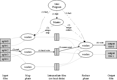
Figure 1 shows the overall flow of a MapReduce operation in our implementation. When the user program calls the MapReduce function, the following sequence of actions occurs (the numbered labels in Figure 1 correspond to the numbers in the list below):
After successful completion, the output of the mapreduce execution is
available in the ![]() output files (one per reduce task, with file
names as specified by the user). Typically, users do not need to
combine these
output files (one per reduce task, with file
names as specified by the user). Typically, users do not need to
combine these ![]() output files into one file - they often pass these
files as input to another MapReduce call, or use them from another
distributed application that is able to deal with input that is
partitioned into multiple files.
output files into one file - they often pass these
files as input to another MapReduce call, or use them from another
distributed application that is able to deal with input that is
partitioned into multiple files.
The master keeps several data structures. For each map task and reduce task, it stores the state (_idle_, _in-progress_, or _completed_), and the identity of the worker machine (for non-idle tasks).
The master is the conduit through which the location of intermediate
file regions is propagated from map tasks to reduce tasks. Therefore,
for each completed map task, the master stores the locations and sizes
of the ![]() intermediate file regions produced by the map task.
Updates to this location and size information are received as map
tasks are completed. The information is pushed incrementally to
workers that have _in-progress_ reduce tasks.
intermediate file regions produced by the map task.
Updates to this location and size information are received as map
tasks are completed. The information is pushed incrementally to
workers that have _in-progress_ reduce tasks.
The master pings every worker periodically. If no response is received from a worker in a certain amount of time, the master marks the worker as failed. Any map tasks completed by the worker are reset back to their initial _idle_ state, and therefore become eligible for scheduling on other workers. Similarly, any map task or reduce task in progress on a failed worker is also reset to _idle_ and becomes eligible for rescheduling.
Completed map tasks are re-executed on a failure because their output is stored on the local disk(s) of the failed machine and is therefore inaccessible. Completed reduce tasks do not need to be re-executed since their output is stored in a global file system.
When a map task is executed first by worker ![]() and then later
executed by worker
and then later
executed by worker ![]() (because
(because ![]() failed), all workers executing
reduce tasks are notified of the re-execution. Any reduce task that
has not already read the data from worker
failed), all workers executing
reduce tasks are notified of the re-execution. Any reduce task that
has not already read the data from worker ![]() will read the data from
worker
will read the data from
worker ![]() .
.
MapReduce is resilient to large-scale worker failures. For example, during one MapReduce operation, network maintenance on a running cluster was causing groups of 80 machines at a time to become unreachable for several minutes. The MapReduce master simply re-executed the work done by the unreachable worker machines, and continued to make forward progress, eventually completing the MapReduce operation.
It is easy to make the master write periodic checkpoints of the master data structures described above. If the master task dies, a new copy can be started from the last checkpointed state. However, given that there is only a single master, its failure is unlikely; therefore our current implementation aborts the MapReduce computation if the master fails. Clients can check for this condition and retry the MapReduce operation if they desire.
When the user-supplied _map_ and _reduce_ operators are deterministic functions of their input values, our distributed implementation produces the same output as would have been produced by a non-faulting sequential execution of the entire program.
We rely on atomic commits of map and reduce task outputs to achieve
this property. Each in-progress task writes its output to private
temporary files. A reduce task produces one such file, and a map task
produces ![]() such files (one per reduce task). When a map task
completes, the worker sends a message to the master and includes the
names of the
such files (one per reduce task). When a map task
completes, the worker sends a message to the master and includes the
names of the ![]() temporary files in the message. If the master
receives a completion message for an already completed map task, it
ignores the message. Otherwise, it records the names of
temporary files in the message. If the master
receives a completion message for an already completed map task, it
ignores the message. Otherwise, it records the names of ![]() files in
a master data structure.
files in
a master data structure.
When a reduce task completes, the reduce worker atomically renames its temporary output file to the final output file. If the same reduce task is executed on multiple machines, multiple rename calls will be executed for the same final output file. We rely on the atomic rename operation provided by the underlying file system to guarantee that the final file system state contains just the data produced by one execution of the reduce task.
The vast majority of our _map_ and _reduce_ operators are
deterministic, and the fact that our semantics are equivalent to a
sequential execution in this case makes it very easy for programmers to
reason about their program's behavior. When the _map_ and/or _reduce_
operators are non-deterministic, we provide weaker but still
reasonable semantics. In the presence of non-deterministic operators,
the output of a particular reduce task ![]() is equivalent to the
output for
is equivalent to the
output for ![]() produced by a sequential execution of the
non-deterministic program. However, the output for a different reduce
task
produced by a sequential execution of the
non-deterministic program. However, the output for a different reduce
task ![]() may correspond to the output for
may correspond to the output for ![]() produced by a
different sequential execution of the non-deterministic program.
produced by a
different sequential execution of the non-deterministic program.
Consider map task ![]() and reduce tasks
and reduce tasks ![]() and
and ![]() . Let
. Let ![]() be the execution of
be the execution of ![]() that committed (there is exactly one such
execution). The weaker semantics arise because
that committed (there is exactly one such
execution). The weaker semantics arise because ![]() may have read
the output produced by one execution of
may have read
the output produced by one execution of ![]() and
and ![]() may have read
the output produced by a different execution of
may have read
the output produced by a different execution of ![]() .
.
Network bandwidth is a relatively scarce resource in our computing environment. We conserve network bandwidth by taking advantage of the fact that the input data (managed by GFS [8]) is stored on the local disks of the machines that make up our cluster. GFS divides each file into 64 MB blocks, and stores several copies of each block (typically 3 copies) on different machines. The MapReduce master takes the location information of the input files into account and attempts to schedule a map task on a machine that contains a replica of the corresponding input data. Failing that, it attempts to schedule a map task near a replica of that task's input data (e.g., on a worker machine that is on the same network switch as the machine containing the data). When running large MapReduce operations on a significant fraction of the workers in a cluster, most input data is read locally and consumes no network bandwidth.
We subdivide the map phase into ![]() pieces and the reduce phase into
pieces and the reduce phase into
![]() pieces, as described above. Ideally,
pieces, as described above. Ideally, ![]() and
and ![]() should be much
larger than the number of worker machines. Having each worker perform
many different tasks improves dynamic load balancing, and also speeds
up recovery when a worker fails: the many map tasks it has
completed can be spread out across all the other worker machines.
should be much
larger than the number of worker machines. Having each worker perform
many different tasks improves dynamic load balancing, and also speeds
up recovery when a worker fails: the many map tasks it has
completed can be spread out across all the other worker machines.
There are practical bounds on how large ![]() and
and ![]() can be in our
implementation, since the master must make
can be in our
implementation, since the master must make ![]() scheduling decisions and keeps
scheduling decisions and keeps ![]() state in memory as described
above. (The constant factors for memory usage are small however:
the
state in memory as described
above. (The constant factors for memory usage are small however:
the ![]() piece of the state consists of approximately one byte of
data per map task/reduce task pair.)
piece of the state consists of approximately one byte of
data per map task/reduce task pair.)
Furthermore, ![]() is often constrained by users because the output of
each reduce task ends up in a separate output file. In practice, we
tend to choose
is often constrained by users because the output of
each reduce task ends up in a separate output file. In practice, we
tend to choose ![]() so that each individual task is roughly 16 MB to 64
MB of input data (so that the locality optimization described above is
most effective), and we make
so that each individual task is roughly 16 MB to 64
MB of input data (so that the locality optimization described above is
most effective), and we make ![]() a small multiple of the number of
worker machines we expect to use. We often perform MapReduce
computations with
a small multiple of the number of
worker machines we expect to use. We often perform MapReduce
computations with ![]() and
and ![]() , using 2,000 worker
machines.
, using 2,000 worker
machines.
One of the common causes that lengthens the total time taken for a MapReduce operation is a ``straggler'': a machine that takes an unusually long time to complete one of the last few map or reduce tasks in the computation. Stragglers can arise for a whole host of reasons. For example, a machine with a bad disk may experience frequent correctable errors that slow its read performance from 30 MB/s to 1 MB/s. The cluster scheduling system may have scheduled other tasks on the machine, causing it to execute the MapReduce code more slowly due to competition for CPU, memory, local disk, or network bandwidth. A recent problem we experienced was a bug in machine initialization code that caused processor caches to be disabled: computations on affected machines slowed down by over a factor of one hundred.
We have a general mechanism to alleviate the problem of stragglers. When a MapReduce operation is close to completion, the master schedules backup executions of the remaining _in-progress_ tasks. The task is marked as completed whenever either the primary or the backup execution completes. We have tuned this mechanism so that it typically increases the computational resources used by the operation by no more than a few percent. We have found that this significantly reduces the time to complete large MapReduce operations. As an example, the sort program described in Section 5.3 takes 44% longer to complete when the backup task mechanism is disabled.
Although the basic functionality provided by simply writing _Map_ and _Reduce_ functions is sufficient for most needs, we have found a few extensions useful. These are described in this section.
The users of MapReduce specify the number of reduce tasks/output files
that they desire (![]() ). Data gets partitioned across these tasks
using a partitioning function on the intermediate key. A default
partitioning function is provided that uses hashing
(e.g. ``
). Data gets partitioned across these tasks
using a partitioning function on the intermediate key. A default
partitioning function is provided that uses hashing
(e.g. ``
![]() ''). This tends to result in fairly
well-balanced partitions. In some cases, however, it is useful to
partition data by some other function of the key. For example,
sometimes the output keys are URLs, and we want all entries for a
single host to end up in the same output file. To support situations
like this, the user of the MapReduce library can provide a special
partitioning function. For example, using
``
''). This tends to result in fairly
well-balanced partitions. In some cases, however, it is useful to
partition data by some other function of the key. For example,
sometimes the output keys are URLs, and we want all entries for a
single host to end up in the same output file. To support situations
like this, the user of the MapReduce library can provide a special
partitioning function. For example, using
``
![]() ''
as the partitioning function causes all URLs from the
same host to end up in the same output file.
''
as the partitioning function causes all URLs from the
same host to end up in the same output file.
We guarantee that within a given partition, the intermediate key/value pairs are processed in increasing key order. This ordering guarantee makes it easy to generate a sorted output file per partition, which is useful when the output file format needs to support efficient random access lookups by key, or users of the output find it convenient to have the data sorted.
In some cases, there is significant repetition in the intermediate keys produced by each map task, and the user-specified _Reduce_ function is commutative and associative. A good example of this is the word counting example in Section 2.1. Since word frequencies tend to follow a Zipf distribution, each map task will produce hundreds or thousands of records of the form <the, 1>. All of these counts will be sent over the network to a single reduce task and then added together by the _Reduce_ function to produce one number. We allow the user to specify an optional _Combiner_ function that does partial merging of this data before it is sent over the network.
The _Combiner_ function is executed on each machine that performs a map task. Typically the same code is used to implement both the combiner and the reduce functions. The only difference between a reduce function and a combiner function is how the MapReduce library handles the output of the function. The output of a reduce function is written to the final output file. The output of a combiner function is written to an intermediate file that will be sent to a reduce task.
Partial combining significantly speeds up certain classes of MapReduce operations. Appendix A contains an example that uses a combiner.
The MapReduce library provides support for reading input data in several different formats. For example, ``text'' mode input treats each line as a key/value pair: the key is the offset in the file and the value is the contents of the line. Another common supported format stores a sequence of key/value pairs sorted by key. Each input type implementation knows how to split itself into meaningful ranges for processing as separate map tasks (e.g. text mode's range splitting ensures that range splits occur only at line boundaries). Users can add support for a new input type by providing an implementation of a simple _reader_ interface, though most users just use one of a small number of predefined input types.
A _reader_ does not necessarily need to provide data read from a file. For example, it is easy to define a _reader_ that reads records from a database, or from data structures mapped in memory.
In a similar fashion, we support a set of output types for producing data in different formats and it is easy for user code to add support for new output types.
In some cases, users of MapReduce have found it convenient to produce auxiliary files as additional outputs from their map and/or reduce operators. We rely on the application writer to make such side-effects atomic and idempotent. Typically the application writes to a temporary file and atomically renames this file once it has been fully generated.
We do not provide support for atomic two-phase commits of multiple output files produced by a single task. Therefore, tasks that produce multiple output files with cross-file consistency requirements should be deterministic. This restriction has never been an issue in practice.
Sometimes there are bugs in user code that cause the _Map_ or _Reduce_ functions to crash deterministically on certain records. Such bugs prevent a MapReduce operation from completing. The usual course of action is to fix the bug, but sometimes this is not feasible; perhaps the bug is in a third-party library for which source code is unavailable. Also, sometimes it is acceptable to ignore a few records, for example when doing statistical analysis on a large data set. We provide an optional mode of execution where the MapReduce library detects which records cause deterministic crashes and skips these records in order to make forward progress.
Each worker process installs a signal handler that catches segmentation violations and bus errors. Before invoking a user _Map_ or _Reduce_ operation, the MapReduce library stores the sequence number of the argument in a global variable. If the user code generates a signal, the signal handler sends a ``last gasp'' UDP packet that contains the sequence number to the MapReduce master. When the master has seen more than one failure on a particular record, it indicates that the record should be skipped when it issues the next re-execution of the corresponding Map or Reduce task.
Debugging problems in _Map_ or _Reduce_ functions can be tricky, since the actual computation happens in a distributed system, often on several thousand machines, with work assignment decisions made dynamically by the master. To help facilitate debugging, profiling, and small-scale testing, we have developed an alternative implementation of the MapReduce library that sequentially executes all of the work for a MapReduce operation on the local machine. Controls are provided to the user so that the computation can be limited to particular map tasks. Users invoke their program with a special flag and can then easily use any debugging or testing tools they find useful (e.g. gdb).
The master runs an internal HTTP server and exports a set of status pages for human consumption. The status pages show the progress of the computation, such as how many tasks have been completed, how many are in progress, bytes of input, bytes of intermediate data, bytes of output, processing rates, etc. The pages also contain links to the standard error and standard output files generated by each task. The user can use this data to predict how long the computation will take, and whether or not more resources should be added to the computation. These pages can also be used to figure out when the computation is much slower than expected.
In addition, the top-level status page shows which workers have failed, and which map and reduce tasks they were processing when they failed. This information is useful when attempting to diagnose bugs in the user code.
The MapReduce library provides a counter facility to count occurrences of various events. For example, user code may want to count total number of words processed or the number of German documents indexed, etc.
To use this facility, user code creates a named counter object and then increments the counter appropriately in the _Map_ and/or _Reduce_ function. For example:
  Counter* uppercase;
  uppercase = GetCounter("uppercase");

  map(String name, String contents):
    for each word w in contents:
      if (IsCapitalized(w)):
        uppercase->Increment();
      EmitIntermediate(w, "1");
The counter values from individual worker machines are periodically propagated to the master (piggybacked on the ping response). The master aggregates the counter values from successful map and reduce tasks and returns them to the user code when the MapReduce operation is completed. The current counter values are also displayed on the master status page so that a human can watch the progress of the live computation. When aggregating counter values, the master eliminates the effects of duplicate executions of the same map or reduce task to avoid double counting. (Duplicate executions can arise from our use of backup tasks and from re-execution of tasks due to failures.)
Some counter values are automatically maintained by the MapReduce library, such as the number of input key/value pairs processed and the number of output key/value pairs produced.
Users have found the counter facility useful for sanity checking the behavior of MapReduce operations. For example, in some MapReduce operations, the user code may want to ensure that the number of output pairs produced exactly equals the number of input pairs processed, or that the fraction of German documents processed is within some tolerable fraction of the total number of documents processed.
In this section we measure the performance of MapReduce on two computations running on a large cluster of machines. One computation searches through approximately one terabyte of data looking for a particular pattern. The other computation sorts approximately one terabyte of data.
These two programs are representative of a large subset of the real programs written by users of MapReduce - one class of programs shuffles data from one representation to another, and another class extracts a small amount of interesting data from a large data set.
All of the programs were executed on a cluster that consisted of approximately 1800 machines. Each machine had two 2GHz Intel Xeon processors with Hyper-Threading enabled, 4GB of memory, two 160GB IDE disks, and a gigabit Ethernet link. The machines were arranged in a two-level tree-shaped switched network with approximately 100-200 Gbps of aggregate bandwidth available at the root. All of the machines were in the same hosting facility and therefore the round-trip time between any pair of machines was less than a millisecond.
Out of the 4GB of memory, approximately 1-1.5GB was reserved by other tasks running on the cluster. The programs were executed on a weekend afternoon, when the CPUs, disks, and network were mostly idle.
|
|
The grep program scans through ![]() 100-byte records,
searching for a relatively rare three-character pattern (the pattern
occurs in 92,337 records). The input is split into approximately 64MB
pieces (
100-byte records,
searching for a relatively rare three-character pattern (the pattern
occurs in 92,337 records). The input is split into approximately 64MB
pieces (![]() ), and the entire output is placed in one file (
), and the entire output is placed in one file (![]() ).
).
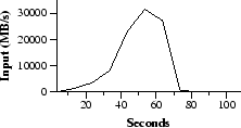
Figure 2 shows the progress of the computation over time. The Y-axis shows the rate at which the input data is scanned. The rate gradually picks up as more machines are assigned to this MapReduce computation, and peaks at over 30 GB/s when 1764 workers have been assigned. As the map tasks finish, the rate starts dropping and hits zero about 80 seconds into the computation. The entire computation takes approximately 150 seconds from start to finish. This includes about a minute of startup overhead. The overhead is due to the propagation of the program to all worker machines, and delays interacting with GFS to open the set of 1000 input files and to get the information needed for the locality optimization.
The sort program sorts ![]() 100-byte records
(approximately 1 terabyte of data). This program is modeled after the
TeraSort benchmark [10].
100-byte records
(approximately 1 terabyte of data). This program is modeled after the
TeraSort benchmark [10].
The sorting program consists of less than 50 lines of user code. A three-line _Map_ function extracts a 10-byte sorting key from a text line and emits the key and the original text line as the intermediate key/value pair. We used a built-in _Identity_ function as the _Reduce_ operator. This functions passes the intermediate key/value pair unchanged as the output key/value pair. The final sorted output is written to a set of 2-way replicated GFS files (i.e., 2 terabytes are written as the output of the program).
As before, the input data is split into 64MB pieces (![]() ). We
partition the sorted output into 4000 files (
). We
partition the sorted output into 4000 files (![]() ). The
partitioning function uses the initial bytes of the key to segregate
it into one of
). The
partitioning function uses the initial bytes of the key to segregate
it into one of ![]() pieces.
pieces.
Our partitioning function for this benchmark has built-in knowledge of the distribution of keys. In a general sorting program, we would add a pre-pass MapReduce operation that would collect a sample of the keys and use the distribution of the sampled keys to compute split-points for the final sorting pass.
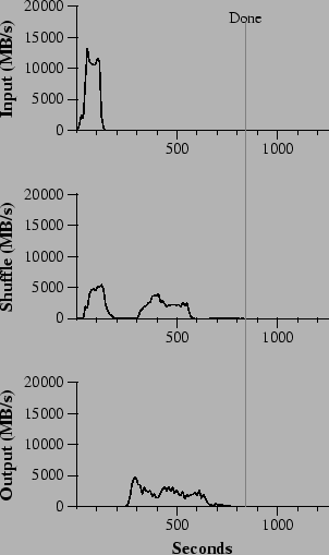
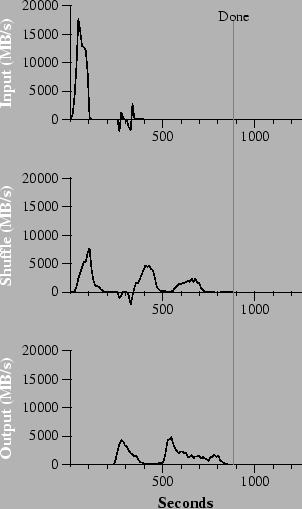
Figure 3 (a) shows the progress of a normal execution of the sort program. The top-left graph shows the rate at which input is read. The rate peaks at about 13 GB/s and dies off fairly quickly since all map tasks finish before 200 seconds have elapsed. Note that the input rate is less than for grep. This is because the sort map tasks spend about half their time and I/O bandwidth writing intermediate output to their local disks. The corresponding intermediate output for grep had negligible size.
The middle-left graph shows the rate at which data is sent over the network from the map tasks to the reduce tasks. This shuffling starts as soon as the first map task completes. The first hump in the graph is for the first batch of approximately 1700 reduce tasks (the entire MapReduce was assigned about 1700 machines, and each machine executes at most one reduce task at a time). Roughly 300 seconds into the computation, some of these first batch of reduce tasks finish and we start shuffling data for the remaining reduce tasks. All of the shuffling is done about 600 seconds into the computation.
The bottom-left graph shows the rate at which sorted data is written to the final output files by the reduce tasks. There is a delay between the end of the first shuffling period and the start of the writing period because the machines are busy sorting the intermediate data. The writes continue at a rate of about 2-4 GB/s for a while. All of the writes finish about 850 seconds into the computation. Including startup overhead, the entire computation takes 891 seconds. This is similar to the current best reported result of 1057 seconds for the TeraSort benchmark [18].
A few things to note: the input rate is higher than the shuffle rate and the output rate because of our locality optimization - most data is read from a local disk and bypasses our relatively bandwidth constrained network. The shuffle rate is higher than the output rate because the output phase writes two copies of the sorted data (we make two replicas of the output for reliability and availability reasons). We write two replicas because that is the mechanism for reliability and availability provided by our underlying file system. Network bandwidth requirements for writing data would be reduced if the underlying file system used erasure coding [14] rather than replication.
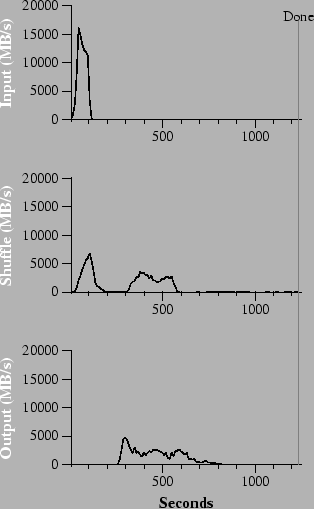
In Figure 3 (b), we show an execution of the sort program with backup tasks disabled. The execution flow is similar to that shown in Figure 3 (a), except that there is a very long tail where hardly any write activity occurs. After 960 seconds, all except 5 of the reduce tasks are completed. However these last few stragglers don't finish until 300 seconds later. The entire computation takes 1283 seconds, an increase of 44% in elapsed time.
In Figure 3 (c), we show an execution of the sort program where we intentionally killed 200 out of 1746 worker processes several minutes into the computation. The underlying cluster scheduler immediately restarted new worker processes on these machines (since only the processes were killed, the machines were still functioning properly).
The worker deaths show up as a negative input rate since some previously completed map work disappears (since the corresponding map workers were killed) and needs to be redone. The re-execution of this map work happens relatively quickly. The entire computation finishes in 933 seconds including startup overhead (just an increase of 5% over the normal execution time).
We wrote the first version of the MapReduce library in February of 2003, and made significant enhancements to it in August of 2003, including the locality optimization, dynamic load balancing of task execution across worker machines, etc. Since that time, we have been pleasantly surprised at how broadly applicable the MapReduce library has been for the kinds of problems we work on. It has been used across a wide range of domains within Google, including:
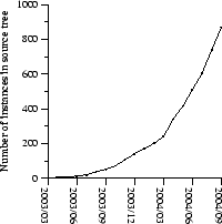
Figure 4 shows the significant growth in the number of separate MapReduce programs checked into our primary source code management system over time, from 0 in early 2003 to almost 900 separate instances as of late September 2004. MapReduce has been so successful because it makes it possible to write a simple program and run it efficiently on a thousand machines in the course of half an hour, greatly speeding up the development and prototyping cycle. Furthermore, it allows programmers who have no experience with distributed and/or parallel systems to exploit large amounts of resources easily.
At the end of each job, the MapReduce library logs statistics about the computational resources used by the job. In Table 1, we show some statistics for a subset of MapReduce jobs run at Google in August 2004.
One of our most significant uses of MapReduce to date has been a complete rewrite of the production indexing system that produces the data structures used for the Google web search service. The indexing system takes as input a large set of documents that have been retrieved by our crawling system, stored as a set of GFS files. The raw contents for these documents are more than 20 terabytes of data. The indexing process runs as a sequence of five to ten MapReduce operations. Using MapReduce (instead of the ad-hoc distributed passes in the prior version of the indexing system) has provided several benefits:
Many systems have provided restricted programming models and used the
restrictions to parallelize the computation automatically. For
example, an associative function can be computed over all prefixes of
an ![]() element array in
element array in ![]() time on
time on ![]() processors using parallel
prefix computations [6,9,13]. MapReduce
can be considered a simplification and distillation of some of these
models based on our experience with large real-world computations.
More significantly, we provide a fault-tolerant implementation that
scales to thousands of processors. In contrast, most of the parallel
processing systems have only been implemented on smaller scales and
leave the details of handling machine failures to the programmer.
processors using parallel
prefix computations [6,9,13]. MapReduce
can be considered a simplification and distillation of some of these
models based on our experience with large real-world computations.
More significantly, we provide a fault-tolerant implementation that
scales to thousands of processors. In contrast, most of the parallel
processing systems have only been implemented on smaller scales and
leave the details of handling machine failures to the programmer.
Bulk Synchronous Programming [17] and some MPI primitives [11] provide higher-level abstractions that make it easier for programmers to write parallel programs. A key difference between these systems and MapReduce is that MapReduce exploits a restricted programming model to parallelize the user program automatically and to provide transparent fault-tolerance.
Our locality optimization draws its inspiration from techniques such as active disks [12,15], where computation is pushed into processing elements that are close to local disks, to reduce the amount of data sent across I/O subsystems or the network. We run on commodity processors to which a small number of disks are directly connected instead of running directly on disk controller processors, but the general approach is similar.
Our backup task mechanism is similar to the eager scheduling mechanism employed in the Charlotte System [3]. One of the shortcomings of simple eager scheduling is that if a given task causes repeated failures, the entire computation fails to complete. We fix some instances of this problem with our mechanism for skipping bad records.
The MapReduce implementation relies on an in-house cluster management system that is responsible for distributing and running user tasks on a large collection of shared machines. Though not the focus of this paper, the cluster management system is similar in spirit to other systems such as Condor [16].
The sorting facility that is a part of the MapReduce library is
similar in operation to NOW-Sort [1]. Source machines
(map workers) partition the data to be sorted and send it to one of
![]() reduce workers. Each reduce worker sorts its data locally (in
memory if possible). Of course NOW-Sort does not have the
user-definable Map and Reduce functions that make our library widely
applicable.
reduce workers. Each reduce worker sorts its data locally (in
memory if possible). Of course NOW-Sort does not have the
user-definable Map and Reduce functions that make our library widely
applicable.
River [2] provides a programming model where processes communicate with each other by sending data over distributed queues. Like MapReduce, the River system tries to provide good average case performance even in the presence of non-uniformities introduced by heterogeneous hardware or system perturbations. River achieves this by careful scheduling of disk and network transfers to achieve balanced completion times. MapReduce has a different approach. By restricting the programming model, the MapReduce framework is able to partition the problem into a large number of fine-grained tasks. These tasks are dynamically scheduled on available workers so that faster workers process more tasks. The restricted programming model also allows us to schedule redundant executions of tasks near the end of the job which greatly reduces completion time in the presence of non-uniformities (such as slow or stuck workers).
BAD-FS [5] has a very different programming model from MapReduce, and unlike MapReduce, is targeted to the execution of jobs across a wide-area network. However, there are two fundamental similarities. (1) Both systems use redundant execution to recover from data loss caused by failures. (2) Both use locality-aware scheduling to reduce the amount of data sent across congested network links.
TACC [7] is a system designed to simplify construction of highly-available networked services. Like MapReduce, it relies on re-execution as a mechanism for implementing fault-tolerance.
The MapReduce programming model has been successfully used at Google for many different purposes. We attribute this success to several reasons. First, the model is easy to use, even for programmers without experience with parallel and distributed systems, since it hides the details of parallelization, fault-tolerance, locality optimization, and load balancing. Second, a large variety of problems are easily expressible as MapReduce computations. For example, MapReduce is used for the generation of data for Google's production web search service, for sorting, for data mining, for machine learning, and many other systems. Third, we have developed an implementation of MapReduce that scales to large clusters of machines comprising thousands of machines. The implementation makes efficient use of these machine resources and therefore is suitable for use on many of the large computational problems encountered at Google.
We have learned several things from this work. First, restricting the programming model makes it easy to parallelize and distribute computations and to make such computations fault-tolerant. Second, network bandwidth is a scarce resource. A number of optimizations in our system are therefore targeted at reducing the amount of data sent across the network: the locality optimization allows us to read data from local disks, and writing a single copy of the intermediate data to local disk saves network bandwidth. Third, redundant execution can be used to reduce the impact of slow machines, and to handle machine failures and data loss.
Josh Levenberg has been instrumental in revising and extending the user-level MapReduce API with a number of new features based on his experience with using MapReduce and other people's suggestions for enhancements. MapReduce reads its input from and writes its output to the Google File System [8]. We would like to thank Mohit Aron, Howard Gobioff, Markus Gutschke, David Kramer, Shun-Tak Leung, and Josh Redstone for their work in developing GFS. We would also like to thank Percy Liang and Olcan Sercinoglu for their work in developing the cluster management system used by MapReduce. Mike Burrows, Wilson Hsieh, Josh Levenberg, Sharon Perl, Rob Pike, and Debby Wallach provided helpful comments on earlier drafts of this paper. The anonymous OSDI reviewers, and our shepherd, Eric Brewer, provided many useful suggestions of areas where the paper could be improved. Finally, we thank all the users of MapReduce within Google's engineering organization for providing helpful feedback, suggestions, and bug reports.
This section contains a program that counts the number of occurrences of each unique word in a set of input files specified on the command line.
#include "mapreduce/mapreduce.h"

// User's map function
class WordCounter : public Mapper {
 public:
  virtual void Map(const MapInput& input) {
    const string& text = input.value();
    const int n = text.size();
    for (int i = 0; i < n; ) {
      // Skip past leading whitespace
      while ((i < n) && isspace(text[i]))
        i++;

      // Find word end
      int start = i;
      while ((i < n) && !isspace(text[i]))
        i++;

      if (start < i)
        Emit(text.substr(start,i-start),"1");
    }
  }
};
REGISTER_MAPPER(WordCounter);

// User's reduce function
class Adder : public Reducer {
  virtual void Reduce(ReduceInput* input) {
    // Iterate over all entries with the
    // same key and add the values
    int64 value = 0;
    while (!input->done()) {
      value += StringToInt(input->value());
      input->NextValue();
    }

    // Emit sum for input->key()
    Emit(IntToString(value));
  }
};
REGISTER_REDUCER(Adder);

int main(int argc, char** argv) {
  ParseCommandLineFlags(argc, argv);

  MapReduceSpecification spec;

  // Store list of input files into "spec"
  for (int i = 1; i < argc; i++) {
    MapReduceInput* input = spec.add_input();
    input->set_format("text");
    input->set_filepattern(argv[i]);
    input->set_mapper_class("WordCounter");
  }

  // Specify the output files:
  //    /gfs/test/freq-00000-of-00100
  //    /gfs/test/freq-00001-of-00100
  //    ...
  MapReduceOutput* out = spec.output();
  out->set_filebase("/gfs/test/freq");
  out->set_num_tasks(100);
  out->set_format("text");
  out->set_reducer_class("Adder");

  // Optional: do partial sums within map
  // tasks to save network bandwidth
  out->set_combiner_class("Adder");

  // Tuning parameters: use at most 2000
  // machines and 100 MB of memory per task
  spec.set_machines(2000);
  spec.set_map_megabytes(100);
  spec.set_reduce_megabytes(100);

  // Now run it
  MapReduceResult result;
  if (!MapReduce(spec, &result)) abort();

  // Done: 'result' structure contains info
  // about counters, time taken, number of
  // machines used, etc.

  return 0;
}
|
This paper was originally published in the
Proceedings of the 6th Symposium on Operating Systems Design and Implementation,
December 6–8, 2004, San Francisco, CA Last changed: 18 Nov. 2004 aw |
|