FAST '05 Paper
[FAST '05 Technical Program]
On multidimensional data and modern disks
Steven W. Schlosser†,
Jiri Schindler‡,
Stratos Papadomanolakis♦,
Minglong Shao♦,
Anastassia Ailamaki♦,
Christos Faloutsos♦,
Gregory R. Ganger♦
Intel Research Pittsburgh†,
EMC Corporation‡,
Carnegie Mellon University♦
Contents
With the deeply-ingrained notion that disks can efficiently access
only one dimensional data, current approaches for mapping
multidimensional data to disk blocks either allow efficient accesses
in only one dimension, trading off the efficiency of accesses in other
dimensions, or equally penalize access to all dimensions. Yet,
existing technology and functions readily available inside disk
firmware can identify non-contiguous logical blocks that preserve
spatial locality of multidimensional datasets. These blocks, which
span on the order of a hundred adjacent tracks, can be accessed with
minimal positioning cost. This paper details these technologies,
analyzes their trends, and shows how they can be exposed to
applications while maintaining existing abstractions. The described
approach can achieve the best possible access efficiency afforded by
the disk technologies: sequential access along primary dimension and
access with minimal positioning cost for all other
dimensions. Experimental evaluation of a prototype implementation
demonstrates a reduction of overall I/O time for multidimensional data
queries between 30% and 50% when compared to existing approaches.
Large, multidimensional datasets are becoming more prevalent in both
scientific and business computing. Applications, such as earthquake
simulation and oil and gas exploration, utilize large
three-dimensional datasets representing the composition of the earth.
Simulation and visualization transform these datasets into four
dimensions, adding time as a component of the data. Conventional
two-dimensional relational databases can be represented as
multidimensional data using online analytical processing (OLAP)
techniques, allowing complex queries for data mining. Queries on this
data are often ad-hoc, making it difficult to optimize for a
particular workload or access pattern. As these datasets grow in size
and popularity, the performance of the applications that access them
growing in importance.
Unfortunately, storage performance for this type of data is often
inadequate, largely due to the one-dimensional abstraction of disk
drives and disk arrays. Today's data placement techniques are
commonly predicated on the assumption that multidimensional data must
be serialized when stored on disk. Put another way, the assumption is
that spatial locality cannot be preserved along all dimensions of the
dataset once it is stored on disk. Various data placement and
indexing techniques have been proposed over the years to optimize
access performance for various data types and query workloads, but
none solve the fundamental problem of preserving locality of
multidimensional data.
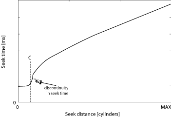
Figure 1: Notional seek curve of a modern disk drive. The
seek time profile of a modern disk drive consists of three distinct
regions. For cylinder distances less than C, the seek time
is constant, followed by a discontinuity. After this point of
discontinuity, the seek time is approximately the square root of the
seek distance. For distances larger than one third of the full seek
distance, the seek time is a linear function of seek distance. To
illustrate the trend more clearly, the X axis is not drawn to scale.
Some recent work has begun to chip away at this
assumption [13,27], showing that locality in
two-dimensional relational databases can be preserved on disk drives,
but we believe that these studies have only scratched the surface of
what is possible given the characteristics and trends of modern disks.
In this paper, we show that modern disk drives can physically
preserve spatial locality for multidimensional data. Our technique
takes advantage of the dramatically higher densities of modern disks,
which have increased the number of tracks that can be accessed within
the time that it takes the disk head to settle on a destination track.
Any of the tracks that can be reached within the settle time can be
accessed for approximately equal cost, which contrasts with the
standard ``rule of thumb'' of disk drive technology that longer seek
distances correspond to longer seek times.
Figure 1 illustrates the basic concept
using a canonical seek curve of a modern disk drive. In contrast to
conventional wisdom, seek time for small distances (i.e., fewer than
C cylinders, as illustrated in the figure) is often a
constant time equal to the time for the disk head to settle on the
destination cylinder. We have found that C is not
trivially small, but can be as high as 100 cylinders in
modern disks. This means that on the order of 100 disk blocks can be
accessed for equal cost from a given starting block. We refer to
these blocks as being adjacent to the starting block,
meaning that any of them can be accessed for equal cost.
In this paper, we explain the adjacency mechanism, detailing the
parameter trends that enable it today and will continue to enable it
into the future. We describe the design and implementation of a
prototype disk array logical volume manager that allows applications
to identify and access adjacent disk blocks, while hiding
extraneous disk-specific details so as to not burden the programmer.
As an example, we also evaluate a data placement technique that maps a
three- and four-dimensional dataset onto the logical volume,
preserving physical locality directly on disk, and improving spatial
query performance by between 30% and 50% over existing data
placements.
The rest of this paper is organized as follows.
Section 2 describes related work.
Section 3 describes details of the adjacency
mechanism, how it can be implemented in modern disks, and historic
and projected disk parameter trends that enable the adjacency
mechanism. Section 4 analyzes data obtained
from measurements of several state-of-the art enterprise-class
SCSI disks to show how their characteristics affect the properties
of the adjacency mechanism. Section 5 shows
how adjacency can be expressed to applications without
burdening them with disk-specific parameters.
Section 6 evaluates the efficiency of adjacent
access on a prototype system using microbenchmarks as well as 3D
and 4D spatial queries.
Effective multidimensional data layout techniques are crucial for the
performance of a wide range of scientific and commercial applications.
We now describe the applications that will benefit from our approach
and show that existing techniques do not address the problem of
preserving the locality of multidimensional data accesses.
Advances in computer hardware and instrumentation allow
high-resolution experiments and simulations that improve our
understanding of complex physical phenomena, from high-energy particle
interactions to combustion and earthquake propagation. The datasets
involved in modern scientific practice are massive and
multidimensional. Modern simulations produce data at the staggering
rate of multiple terabytes per day [21], while high energy
collision experiments at CERN are expected to generate raw data of a
petabyte scale [33]. Realizing the big benefits of the
emerging data-driven scientific paradigm heavily depends on our
ability to efficiently process these large-scale datasets.
Simulation applications are a great example for the storage and
data management challenges posed by large-scale scientific
datasets. Earthquake simulations [2] compute the
propagation of an earthquake wave over time, given the geological
properties of a ground region and the initial conditions. The
problem is discretized by sampling the ground at a collection of
points and the earthquake's duration as a set of time-steps. The
simulator then computes physical parameters (like ground velocity)
for each discrete ground point and for each time
step. Post-processing and visualization applications extract
useful information from the output.
The difficulties in efficiently processing simulation output
datasets lie in their volume and their multidimensional
nature. Storing one time-step of output requires many gigabytes, while
a typical simulation generates about 25,000 such time-steps
[40]. An earthquake simulation dataset is four-dimensional: it
encodes three-dimensional information (the 3D coordinates of the
sample points) at each time-step. Post-processing or visualization
applications query the output, selecting the simulation results that
correspond to ranges of the 4D coordinate space. As an example of such
range queries, consider a ``space-varying'' query that retrieves
the simulated values for all the ground points falling within a given
3D region for only a single time-step. Similarly, ``time-varying''
queries generate waveforms by querying the simulated values for a
single point, but for a range of time-steps.
Unfortunately, naive data layout schemes lead to sub-optimal I/O
performance. Optimizing for a given class of queries (e.g., the 3D
spatial ranges), results in random accesses along the other dimensions
(e.g., the time dimension). Due to the absence of an appropriate disk
layout scheme, I/O performance is the bottleneck in earthquake
simulation applications [40].
Organizing multidimensional data for efficient accesses is a core
problem for several other scientific applications. High energy
physics experiments will produce petabyte-scale datasets with hundreds
of dimensions [33]. Astronomy databases like the Sloan
Digital Sky Survey [15] record astronomical objects using
several other attributes besides their coordinates (brightness in
various wavelengths, redshifts, etc.). The data layout problem becomes
more complex with an increasing number of dimensions because there are
more query classes to be accommodated.
In addition to data-intensive science applications, large-scale
multidimensional datasets are typically used in On-Line Analytical
Processing (OLAP) settings [14,34,39]. OLAP applications
perform complex queries on large volumes of financial transactions
data in order to identify sales trends and support
decision-making. OLAP datasets have large numbers of dimensions,
corresponding, for example, to product and customer
characteristics, and to the time and geographic location of a
sale. Performance of complex multidimensional analysis queries is
critical for the success of OLAP and a large number of techniques
have been proposed for organizing and indexing multidimensional
OLAP data [7, 18, 32, 41].
Efficient multidimensional data access relies on maintaining
locality so that ``neighboring'' objects in the multidimensional
(logical) space are stored in ``neighboring'' disk
locations. Existing multidimensional layout techniques are based
on the standard linear disk abstraction. Therefore, to take
advantage of the efficient sequential disk access, neighboring
objects in the multidimensional space must be stored in disk
blocks with similar logical block numbers (LBNs). Space-filling
curves, such as the Hilbert curve [17],
Z-ordering [22] and Gray-coding [10] are mathematical constructs that map
multidimensional points to a 1D (linear) space, so that nearby
objects in the logical space are as close in the linear ordering
as possible.
Data placement techniques that use space-filling curves rely on a
simplified linear disk model, ignoring low-level details of disk
performance. The resulting linear mapping schemes break
sequential disk access, which can no longer be used for scans
along any dimension, only to ensure that range queries do not
result in completely random I/O. Furthermore, as analysis [20] and our experiments suggest, the ability of
space-filling curves to keep neighbors in any dimensions
physically close on the disk deteriorates rapidly as the number of
dimensions increases. Our work revisits the simplistic disk model
and removes the need for linear mappings. The resulting layout
schemes maintain sequential disk bandwidth, while providing
efficient access along any dimension, even for datasets with large
dimensionality.
Besides space-filling curves, other approaches rely on parallel
I/O to multiple disks. Declustering schemes [1,4,5,11,19,23]
partition the logical multidimensional space across multiple
disks, so that range queries can take advantage of the aggregate
bandwidth available.
The need to efficiently support multidimensional queries has led
to a large body of work on indexing. Multidimensional indexes like
the R-tree [16] and its variants are
disk-resident data structures that provide fast access to the data
objects satisfying a range query. With an appropriate index, query
processing requires only a fraction of disk block accesses,
compared to the alternative of exhaustively searching the entire
dataset. The focus of multidimensional indexing research is on
minimizing the number of disk pages required for answering a given
class of queries [12].
Our work on disk layout for multidimensional datasets differs from
indexing. It improves the performance of retrieving the data
objects that match a given input query and not the efficiency of
identifying those objects. For example, a range query on a dataset
supported by an R-tree can result in a large number of data objects
that must be retrieved. Without an appropriate data layout scheme, the
data objects are likely to reside in separate pages at random disk
locations. After using the index to identify the data objects,
fetching them from the disk will have sub-optimal, random access
performance. Multidimensional indexing techniques are independent of
the underlying data layout and do not address the problem of
maintaining access locality.
Recently, researchers have focused on the lower level of the
storage system in an attempt to improve performance of
multidimensional queries [13, 27, 28, 38].
Part of the work revisits the simple disk abstraction and proposes
to expand the storage interfaces so that the applications can be
more intelligent. Schindler et al. [26]
explored aligning accesses to disk drive track-boundaries to get
rid of rotational latency. Gorbatenko et al. [13] and Schindler et al. [27] proposed a secondary dimension on disks, which
they utilized to create a more flexible database page
layout [30] for two-dimensional
tables. Others have studied the opportunities of building two
dimensional structures to support database applications with new
alternative devices, such as MEMS-based storage devices [28, 38]. The work described in
this paper challenges the underlying assumption of much of this
previous work by showing that the characteristics of modern disk
drives allow for efficient access to multiple dimensions, rather
than just one or two.
The established view is that disk drives can efficiently access only
one-dimensional data mapped to sequential logical blocks. This notion
is further reinforced by the linear abstraction of disk drives as a
sequence of fixed-size blocks. Behind this interface, disks use
various techniques to further optimize for such sequential
accesses. However, modern disk drives can allow for efficient access
in more than one dimension. This fundamental change is based on two
observations of technological trends in modern disks:
- Short seeks of up to some cylinder distance, C, are
dominated by the time the head needs to settle on a new track;
- Firmware features internal to the disk can identify and thus
access blocks that require no rotational latency after a seek.
By combining these two observations, it is possible to construct
access patterns for efficient access to multidimensional data sets
despite the current linear abstractions of storage systems.
This section describes the technical underpinnings of the mechanism
that we exploit to preserve locality of multidimensional data on
disks. We begin by describing some background of the mechanical
operation of disks. We then analyze the technology trends of the
relevant drive parameters, showing how the mechanism is enabled today
and will continue to be enabled in future disks. Lastly, we combine
the two to show how the mechanism itself works.
Positioning To service a request for data access, the disk
must position the read/write head to the physical location where the
data resides. First, it must move a set of arms to the desired
cylinder, in a motion called seeking. Once the set of arms, each
equipped with a distinct head for each surface, is positioned near the
desired track, the head has to settle in the center of the
track. After the head is settled, the disk has to wait for the desired
sector to rotate underneath the stationary head before accessing
it. Thus, the total positioning time is the sum of the seek time,
settle time, and rotational latency components.
The dominant component of the total positioning time depends on the
access pattern (i.e., the location of the previous request with
respect to the next one). If these requests are to two neighboring
sectors on the same track, no positioning overhead is incurred in servicing the
second one. This is referred to as sequential access. When two
requests are located on two adjoining tracks, the disk may incur
settle time and some rotational latency. Finally, if the two requests
are located at non-adjoining tracks, the disk may incur a seek, settle
time, and possibly some rotational latency.
There are two possible definitions of adjoining tracks. They can be
either two tracks with the same radius on different surfaces, or two
neighboring tracks with different radii on the same surface. In the
first case, different heads must be used to access the two tracks; in the second
case, the same head is used for both. In both cases, the disk will
have to settle the head above the correct track. In the former case,
the settle time is incurred because (i) the two tracks on the two
surfaces may not be perfectly aligned or round (called run out), (ii)
the individual heads may not be perfectly stacked, and/or (iii) the
arms may not be stationary (as any non-rigid body, they oscillate
slightly). The former case is referred to as head switch
between tracks of the same cylinder, while the latter is called
a one cylinder seek.
Request scheduling Disk drives use variants of shortest
positioning time first (SPTF) request schedulers [29,36], which determine the
optimal order in which outstanding requests should be serviced by
minimizing the sum of seek/settle time and rotational latency. To
calculate the positioning cost, a scheduler must first determine
the physical locations (i.e., <cylinder, head, sector
offset>) of each request. It then uses seek time estimators
encoded in the firmware routines to calculate the seek time and
calculates residual rotational latency after a seek based on the
offset of the two requests.
Layout Disks map sequential LBNs to adjoining sectors on the same
track. When these sectors are exhausted, the next LBN is mapped to
a specific sector on the adjoining track to minimize the positioning
cost (i.e., head switch or seek to the next cylinder). Hence, there is
some rotational offset between the last LBN on one track and
the next LBN on the next track. Depending on which adjoining track
is chosen for the next LBN, this offset is referred to as track
skew or cylinder skew.
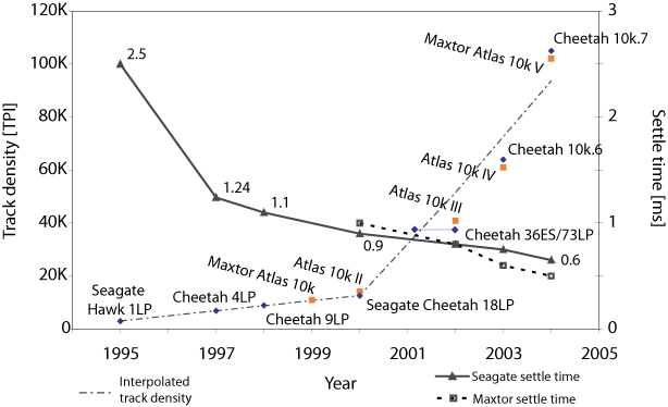
Figure 2:Disk trends for 10,000 RPM disks. Notice the dramatic
increase in track density, measured in Tracks Per Inch (TPI), since
2000, while in the same period, head switch/settle time has improved
only marginally.
The key to our method of enabling multidimensional access on disks is
the relationship between two technology trends over the last decade:
(1) the time for the disk head to settle at the end of a seek has
remained largely constant, and (2) track density has increased
dramatically. Figure 2 shows a graph of both
trends for two families of (mostly) 10,000 RPM
enterprise-class disks from two vendors, Seagate and Maxtor.
The growth of track density, measured in tracks per inch (TPI),
has been one of the strongest trends in disk drive technology.
Over the past decade, while settle time has decreased only by a
factor of 5 [3], track densities
experienced 35 fold increase, as shown in Figure 2. As track density continues to grow while
settle time improves very little, more cylinders can be accessed
in a given amount of time. With all else being equal, more data in
the same physical area can be accessed in the same amount of time.
However, increasing track density negatively impacts the settle
time. With larger TPI, higher-precision controls are required,
diminishing the improvements in settle time due to other factors.
There are other factors that improve seek time such as using
smaller platters [3], but these affect long
and full-strobe seeks, whereas we focus on short-distance seeks.
In the past, the seek time for short distances between one and,
say, L cylinders was approximately the square root of the seek
distance [24]. However, the technology
trends illustrated in Figure 2 lead to seek
times that are nearly constant for distances of up to C
cylinders, and which then increase as before for distances above
C cylinders, as illustrated in Figure 1. Seeks of up to C cylinders are
dominated by the time it takes a disk head to settle on the new
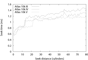
track. These properties are confirmed by looking at the seek
curve measured from a real disk, shown in Figure 3. The graph shows the seek curve for a Maxtor
Atlas 10k III, a 10,000 RPM disk introduced in 2002. For this
disk, C=12 and settle time is around 0.8 ms. For
clarity, the graph shows seek time for distances up to 80
cylinders, even though it has over 31,000 cylinders in total (see
Table 1).
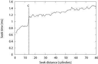
Figure 3:Atlas 10kIII seek curve. First 80 cylinders.
| Model |
Year |
TPI |
Cylinders |
Surfaces |
Max. Cap. |
1-cyl seek |
Full seek |
| Maxtor |
Atlas 10k II |
2000 |
14200 |
17337 |
20 |
73 GB |
1 ms |
12.0 ms |
| Atlas 10k III |
2002 |
40000 |
31002 |
8 |
73 GB |
0.8 ms |
11.0 ms |
| Atlas 10k IV |
2003 |
61000 |
49070 |
8 |
147 GB |
0.6 ms |
12.0 ms |
| Atlas 10k V |
2004 |
102000 |
81782 |
8 |
300 GB |
0.5 ms |
12.0 ms |
| Atlas 15k II |
2004 |
unknown |
48242 |
8 |
147 GB |
0.5 ms |
8.0 ms |
| Seagate |
Cheetah 4LP |
1997 |
6932 |
6526 |
8 |
4.5 GB |
1.24 ms |
19.2 ms |
| Cheetah 36ES |
2001 |
38000 |
26302 |
4 |
36 GB |
0.9 ms |
11.0 ms |
| Cheetah 73LP |
2002 |
38000 |
29549 |
8 |
73 GB |
0.8 ms |
9.8 ms |
| Cheetah 10k.6 |
2003 |
64000 |
49855 |
8 |
147 GB |
0.75 ms |
10.0 ms |
| Cheetah 10k.7 |
2004 |
105000 |
90774 |
8 |
300 GB |
0.65 ms |
10.7 ms |
| Cheetah 15k.4 |
2004 |
85000 |
50864 |
8 |
147 GB |
0.45 ms |
7.9 ms |
Table 1: Disk characteristics. Data taken from
manufacturers' specification sheets. The listed seek times are
for writes.
While settle time has always been a factor in positioning disk heads,
the dramatic increase in bit density over the last decade has brought
it to the fore, as shown in Figure 2. At lower
track densities (i.e., for disks introduced before 2000), only a
single cylinder can be reached within a constant settle time. However,
with the large increase in TPI since 2000, up to C can now
be reached. Section 4.3 examines seek
curves for more disks.
 |
 |
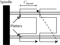 |
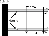
| (a) L-0: traditional. |
(b) L-1: cylinder serpentine. |
(c) L-2: surface serpentine. |
Figure 4: Layout mappings adopted by various disk drives.
The increasing track density also influences how data is laid out on
the disk. While in the past, head switches would be typically faster
than cylinder switches, it is the other way around for today's
disks. With increasing TPI, settling on the correct track with a
different head/arm takes more time than simply settling on the
adjoining track with the same head/arm assembly.
Disks used to lay out data first across all tracks of the same
cylinder before moving to the next one, whereas most recent disks
``stay'' on the same surface for a number of cylinders, say
Clayout,
and move inward before switching to the next surface
and going back. This mapping, which we term
surface serpentine, also leverages the fact that seeks of up
to C cylinders take a (nearly) constant amount of time. Put
differently, the choice of Clayout
must ensure that sequential accesses are still efficient even when
two consecutive LBNs are mapped to tracks Clayout cylinders away.
Figure 4 depicts the different approaches to
mapping LBNs onto disk tracks.
The combination of rapidly increasing track densities and slowly
decreasing settle time leads to the seek curves shown above in
which one of C neighboring cylinders can be accessed from a
given starting point for equal cost. Each of these cylinders is
composed of R tracks, and so, by extension, there are d = R
× C tracks that can be accessed from that starting point
for equal cost. The values of C and d are related very
simply, but we differentiate them to illuminate a subtle, but
important, detail.
The value of C is a measure of how far the disk head
can move (in cylinders) within the settle period, while the value of
d is used to enumerate the number of adjacent blocks that
can be accessed within those cylinders. While each of these d
tracks contain many disk blocks, there is one block on each track that
can be accessed immediately after the head settles on the destination
track, with no additional rotational latency. We identify these
blocks as being adjacent to the starting block.
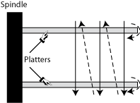
Figure 5 shows a drawing of the layout of
adjacent blocks on disk. For a given starting block, there are
d adjacent disk blocks, one in each of the d
adjacent tracks. For simplicity, we show a disk with only one
surface, so, in this case, R is one, and d equals
C. During the settle time, the disk rotates by a fixed
number of degrees, W, determined by the ratio of the settle
time to the rotational period of the disk. For example, with settle
time of 1 ms and the rotational period of 6 ms
(i.e., for a 10,000 RPM disk), W = 60°.
Therefore, all adjacent blocks have the same angular (physical)
offset from the starting block.
As settle time is not entirely deterministic (i.e., due to
external vibrations or thermal expansion), it is useful to add
some extra conservatism to W to avoid rotational misses, which
lead to long delays. Adding conservatism to the value of W
increases the number of tracks, d, that can be accessed within the
settle time at the cost of added rotational latency. In practice,
disks also add some conservatism to the best-case settle time when
determining cylinder and track skews for mapping LBNs to physical
locations. For our example Atlas 10k III disk, the cylinder and
track skews are 61° and 68°, respectively, or 1.031 ms and
1.141 ms, even though the measured settle time is less than 0.8
ms. This extra buffer of about 14° ensures that the disk will
not miss a rotation during sequential access when going from one
track to the next.
Note that depending on the mapping of logical blocks (LBNs) to
physical locations these blocks can appear to an application either
sequential or non-contiguous. The choice is simply based on how a
particular disk drive does its low-level logical-to-physical
mapping. For example, a pair of sequential LBNs mapped to two
different tracks or cylinders are still adjacent, according to our
definition, as are two specific non-contiguous LBNs mapped to two
nearby tracks.
Accessing successive adjacent disk blocks enables
semi-sequential disk access [13,27], which is the second-most efficient disk
access method after pure sequential access. The delay between
each access is equal to a disk head settle time, which is the
minimum mechanical positioning delay the disk can offer. However,
the semi-sequential access introduced previously utilizes only one
of the adjacent blocks for efficiently accessing 2D data
structures. This work shows how to use up to d adjacent blocks to
improve access efficiency for multidimensional datasets.
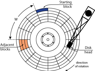
Figure 5:Location of adjacent blocks. W = 67.5° and C = 3.
The previous section defined the adjacency relationship and
identified the disk characteristics which enable access to adjacent
blocks. We now describe two methods for determining the value of
d. The first method we use analyzes the extracted seek curves
and drive parameters to arrive at an estimate for C (and,
by extension, d), and the second method empirically measures
d directly. We evaluate and cross-validate both methods for a
set of disk drives from two different vendors.
All experiments described here are conducted on a two-way 1.7 GHz
Pentium 4 Xeon workstation running Linux kernel 2.4.24. The
machine has 1024 MB of main memory and is equipped with one
Adaptec Ultra160 Wide SCSI adapter connecting the disks. For our
experiments, some of our disks have fewer platters than the
maximum supported, which are listed in Table 1. Most enterprise drives are sold in families
supporting a range of capacities, in which the only difference is
the number of platters in the drive. Specifically, our Cheetah
36ES and Atlas 10k III have two platters, while the Atlas 10k IV,
Atlas 10k V, Cheetah 10k.7, and Cheetah 15k.4 disks have only one
platter. All but one disk have the same total capacity of 36.7 GB;
the Cheetah 10k.7 is a 73 GB disk. Requests are issued to the
disks via the Linux SCSI Generic driver and are timed using the
CPU's cycle counter. All disks had their default cache mode page
settings with both read and write cache enabled.
 |
 |
| (a) Recent Maxtor enterprise-class disks |
(b) Recent Seagate enterprise-class disks |
Figure 6: Measured seek profiles. Only the first 80
cylinders are shown.
To determine the proper values of C and d based on
the disk's characteristics, we need to measure its seek profile. Since
we do not have access to the disk firmware, we have to determine it
empirically. We first obtain mappings of each LBN to its physical
location, given by the <cylinder, head, sector>
tuple. We use the SCSI address translation mode page (0x40h) and
Mode Select command. With a complete layout map, we can
choose a pair of tracks for the desired seek distance and measure how
long it takes to seek from one to the other.
To measure seek time, we choose a pair of cylinders separated by the
desired distance, issue a pair of read commands to sectors in those
cylinders and measure the time between their completions. We choose a
fixed LBN on the source track and successively change the value of
the LBN on the second track, each time issuing a pair of requests,
until we find at the lowest time between request completions. This
technique is called the Minimal Time Between Request Completions
(MTBRC) [37]. The seek time we report is the average
of 6 trials of MTBRC, each with randomly-chosen starting locations
spread across the entire disk. Note that the MTBRC measurement
subtracts the time to read the second sector as well as bus and system
overheads [37].
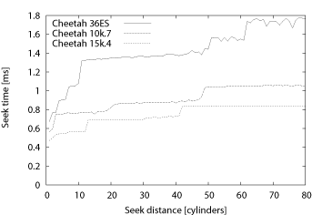
The first method we use to determine C (and thus d) is
based on analyzing the seek profile of a disk. Figure 6 shows seek profiles of the disk drives we
evaluated for small cylinder distances. Note that extracted
profiles have very similar shape, especially among drives from the
same vendor. The one-cylinder seek time is the lowest, as
expected. For distances of two and more cylinders, the seek time
rises rapidly for a few cylinders, but then levels off for several
cylinders before it experiences a large increase between distance
of i and i+1 cylinders. After this inflection point,
which is C, seek time rises gradually with increasing seek
distance.
Note that the seek profile of some disks have more than one
``plateau'' and, thus, several possible values of C. When
determining our value of C we chose the discontinuity point
where seek times after the distance of C are at least 80%
more that the one-cylinder seek time, while seek times of up to
C are at most 60% larger than the one-cylinder seek time.
Note that this is just one way of choosing the appropriate value of
C. In practice, disk designers are likely to choose a value
manually based on the physical disk parameters, just as they choose
the value of track and cylinder skew. In either case, the choice of
C is a trade-off between larger value of d (which
increases the number of potential dimensions that can be accessed
efficiently), and the efficiency of accesses to individual adjacent
blocks.
Using their measured seek curves, we now determine suitable values of
C for six recent disk drives. Recall that C is
the maximal seek distance in cylinders for which positioning time is
(nearly) constant. Table 2 lists the value for each
disk drive determined as the inflection point/discontinuity in the
seek profile. The other pair of numbers in the table shows the
percentage difference between seek time for distance of 1 cylinder and
the distance of respectively C and C+1
cylinders, highlighting this discontinuity.
First, as expected, for more recent disk drives the value of
C increases. Second, the difference between one-cylinder
and C-cylinder seek times is about 50%. And finally, the
difference in seek time between a one- and C+1-cylinder
seek is significant: between 1.7× and 2× the value of
the one-cylinder seek.
Once we have determined a value for C, we simply multiply
by the number of surfaces in the disk to arrive at d.
Figure 7 depicts the values of d for our
disks. For each of the disks, we use the value of C from
Table 2 and multiply it by the maximal number of
surfaces each disk can have. From Table 1, for all
but the Cheetah 36ES, R = 8. We plot the value of
d as a function of year when the particular disk model was
introduced. For years with multiple disks, we average the value of
d across all analyzed disk models. Confirming our trend
analysis, the value of d increases from 40 in year 2001 to
almost 300 in year 2004. Recall that the value of d is
proportional to the number of surfaces in the disk, R,
and that the lower-capacity versions of the disk drives (such as those
in our experiments) will have smaller values of d than those
with more platters.
|
1-cyl seek diff. vs. |
| Disk model |
Year |
C |
C-cyl |
(C+1)-cyl |
| Atlas 10k III |
2002 |
13 |
38% |
76% |
| Atlas 10k IV |
2003 |
12 |
52% |
98% |
| Atlas 10k V |
2004 |
21 |
55% |
91% |
| Cheetah 36ES |
2001 |
10 |
59% |
94% |
| Cheetah 10k.7 |
2004 |
49 |
44% |
80% |
| Cheetah 15k.4 |
2004 |
42 |
55% |
78% |
Table 2: Estimated values of C based on seek
profiles. The seek times compare the extracted value of
1-cylinder seek and C-cylinder seek. The last column lists
the percentage increase between 1-cylinder and C-cylinder
seek time.
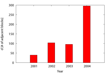
Figure 7: The trend in estimated value of d. The reported values
are based on our estimated values of C multiplied by the disk's
maximal number of surfaces. For years where we measured data from
more than one disk model, we report the average value of d.
We now verify our previous method of determining C by
measuring it directly. We measure the value for d rather than
C, but, of course, C can easily be determined by
dividing d by the number of surfaces in the disk,
R. We use the low-level layout model and the value of
W to identify those blocks that are adjacent to the
starting block. The experiment chooses a random starting block and a
destination block which is i tracks away and is skewed by
W degrees relative to the starting block.
We issue the two requests to the disk simultaneously and measure the
response time of each one individually. If the difference in response
time is equal to the settle time of the disk, then the two blocks are
truly adjacent, and i < d. We increase i until the
response time of the second request increases significantly, beyond
the rotational period of the disk. This value of i is the maximum
distance that the disk head can move and still access adjacent
blocks without missing rotations, so d = i-1.
Adding conservatism to the rotational offset, W, provides a
useful buffer because of nondeterminism in the seek time. We found
this to be especially true when experimenting with real disks, so our
baseline values for W include and aggressive value of
10° for conservatism. Recall that the Atlas 10kIII layout, for
example, uses a buffer of 14° for track and cylinder skews.
Larger conservatism can increase the value of d at the expense
of additional rotational latency and, hence, lower semi-sequential
efficiency. Conceptually, this is analogous to moving to the right
along the seek profile past the discontinuity point. Larger values of
d, in turn, allow mappings of data sets with many more
dimensions, while maintaining the same efficiency for accesses to all
N-1 dimensions. Even though, more conservatism (and larger d)
lowers the achieved semi-sequential bandwidth, it considerably increases
the value of d as illustrated in
Figure 8b.
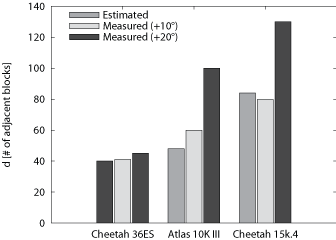
Figure 8a shows the comparison between the value
of d based on our seek profile estimates of C
reported in Table 2 and our measured values using
the above approach. For each disk, we show three bars. The first bar,
labeled ``Estimated'', is the value of the estimated d. The
second and third bar, labeled ``Measured (+10°)'' and
``Measured (+20°)'', show the measured value with a
conservatism of 10° and 20°, respectively, added to
W. the ``Estimated'' values are based on our measurements
from our disks, which have fewer platters that the models reported in
Table 1. In contrast, the values reported in
Figure 7 are based on disks with maximal
capacities.
 |
| Disk model |
W |
Extra |
d |
Access time |
| Atlas 10kIII |
68° |
0° |
25 |
0.95 ms |
|
|
10° |
60 |
1.00 ms |
|
|
20° |
100 |
1.25 ms |
| Cheetah 36ES |
59° |
0° |
20 |
0.85 ms |
|
|
10° |
35 |
1.00 ms |
|
|
20° |
45 |
1.20 ms |
| Cheetah 15k.4 |
70° |
0° |
18 |
0.85 ms |
|
|
10° |
80 |
0.85 ms |
|
|
30° |
130 |
0.85 ms |
|
| (a) Comparison of estimated and measured d |
(b) Increasing conservatism increases
d and access time. |
Figure 8: Comparison of estimated and measured d.
A key feature of adjacent blocks is that, by definition, they can
be accessed immediately after the disk head settles, without any
rotational latency. To quantify the benefits of eliminating
rotational latency, we compare adjacent access to simple nearby
access within d tracks. Without explicit knowledge of
adjacency, accessing each pair of nearby blocks will incur, on
average, rotational latency of half a revolution, in addition to the
seek time equivalent to the settle time. If these blocks are
specifically chosen to be adjacent, then the rotational latency is
eliminated and the access is much more efficient.
As shown in Figure 9, adjacent access
outperforms nearby access by a factor of 4 thanks to the elimination
of all rotational latency Additionally, the access time for the nearby
case varies considerably due to variable rotational latency, while the
access time variability is much smaller for the Adjacent case; it
entirely due to the difference in seek time within the C
cylinders, as depicted by the error bars.
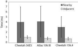
Figure 9: Quantifying access times. This graph compares the access
times to blocks located within C cylinders. For the first
two disks, the average rotational latency is 3 ms, for
Cheetah 15k.4, it is 2 ms.
The previous sections detailed the principles behind efficient access
to d adjacent blocks and demonstrated that existing functions
inside disk firmware (e.g., request schedulers) can readily identify
and access these blocks. However, today's interfaces do not expose
these blocks outside the disk. This section presents the method we
use for exposing adjacent blocks so that applications can use them
for efficient access to multidimensional data. It first describes how
individual disks can cleanly expose adjacent blocks, and then shows
how to combine such information from individual disks comprising a
logical volume and expose it using the same abstractions.
To allow for efficient access, the linear abstraction of disk drives
sets an explicit contract between contiguous LBNs. To extend
efficient access to adjacent blocks, we need to expose explicit
relationships among the set of adjacent LBNs that are
non-contiguous.
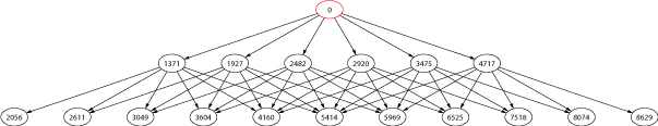
Figure 10: Adjacency graph for LBN 0 of Atlas 10k III. Only two
levels adjacent blocks are shown. The LBNs are shown inside nodes.
To expose the adjacency relationships, we need to augment the
existing interface with one function, here called GETADJACENT.
Given an LBN, this function returns a list of adjacent LBNs
and can be implemented similarly to a LBN-to-physical address
translation, i.e., a vendor-specific SCSI mode page accessed with the
MODE SELECT command. The application need not know the
reasons how or why the returned d disk blocks are adjacent,
it just needs to have them identified through the GETADJACENT
function.
A useful (conceptual) way to express the adjacency relationships
between disk blocks is by constructing adjacency graphs, such as
that shown in Figure 10. The graph nodes
represent disk blocks and the edges connect blocks that are
adjacent. The graph in the figure shows two levels of
adjacency: the root node is the starting block, the nodes in the
intermediate level are adjacent to that block, and the nodes in the
bottom level are adjacent to the blocks in the intermediate level.
Note that adjacent sets of adjacent blocks (i.e., those at the
bottom level of the graph) overlap. For brevity, the graph shows only
the first 6 adjacent blocks (i.e., d = 6), even though
d is considerably larger for this disk, as described in
Section 4. With the concept of adjacent blocks,
applications can lay out and access multidimensional data with the
existing 1D abstraction of the disk. This is possible through explicit
mapping of particular points in the data's multidimensional space to
particular LBNs identified by the disk drive.
Since current disk drives do not expose adjacent blocks and we do
not have access to disk firmware to make the necessary
modifications, we now describe an algorithm for identifying them
in the absence of the proper storage interface functions. The
algorithm uses a detailed model of low-level disk layout borrowed
from a storage system simulator called DiskSim [8]. The parameters can be extracted from SCSI
disks by previously published methods [25,35,37].
The algorithm uses two functions that abstract the disk-specific
details of the disk model: GETSKEW(lbn), which returns
the physical angle between the physical location of an LBN on the
disk and a ``zero'' position, and
GETTRACKBOUNDARIES(lbn), which returns the first and the
last LBN at the ends of the track containing lbn.
For convenience, the algorithm also defines two parameters. First,
the parameter T is the number of disk blocks per track and can be
found by calling GETTRACKBOUNDARIES, and subtracting the low LBN
from the high LBN. Of course, the value of T varies across zones
of an individual disk, and will have to be determined for each call to
GETADJACENT. Second, the parameter W defines the
angle between a starting block and its adjacent blocks. This angle
can be found by calling the GETSKEW function twice for two
consecutive LBNs mapped to two different tracks and computing the
difference; disks skew the mapping of LBNs on consecutive tracks by
W degrees to account for settle time and to optimize
sequential access.
    /* Find an LBN adjacent to lbn and step tracks away */

    L := GETADJACENT(lbn,step):
      /* Find the required skew of target LBN */
      target_skew := (GETSKEW(lbn) + W) mod 360

      /* Find the first LBN in target track */
      base_lbn := lbn + (step × T)
      {low, high} := GETTRACKBOUNDARIES(base_lbn)

      /* Find the minimum skew of target track */
      low_skew := GETSKEW(low)

      /* Find the offset of target LBN from the start of target track */
      if (target_skew > low_skew) then
         offset_skew := target_skew - low_skew
      else
         offset_skew := target_skew - low_skew + 360
      end if

      /* Convert the offset skew into LBNs */
      offset_lbns := (offset_skew / 360) × T
      RETURN(low + offset_lbns)

    /* Find the physical skew of lbn, measured in degrees */
    A := GETSKEW(lbn)

    /* Find the boundaries of the track containing lbn */
    {L, H} := GETTRACKBOUNDARIES(lbn)

    T:  Track length - varies across zones of the disk
    W:  Skew to add between adjacent blocks, measured in degrees
|
Figure 11: Algorithm for the GETADJACENT function.
The GETADJACENT algorithm, shown in Figure 11, takes as input a starting LBN (lbn)
and finds the adjacent LBN that is W degrees ahead and
step tracks away. Every disk block has an adjacent block
within the d closest tracks, so the entire set of adjacent blocks
is found by calling GETADJACENT for increasing values of
step from 1 to d.
So far, we have discussed how to expose adjacent blocks to
applications from a single disk drive. However, large storage systems
combine multiple disks into logical volumes. From our perspective, a
logical volume manager (LVM) adds nothing more than a level of
indirection through mapping of a volume LBN (VLBN) to the
LBNs of individual disks (DLBN). Given a set of adjacent
blocks, an LVM can choose an explicit grouping of LBNs across all
underlying k disks. The d VLBNs exposed via
GETADJACENT are the adjacent blocks of a particular disk's
DLBN mapped to a given VLBN by the LVM. To an application, a
multi-disk logical volume will appear as a (bigger and faster) disk,
whose adjacent blocks set has cardinality d.
Since existing disks do not implement the GETADJACENT and
GETTRACKBOUNDARIES functions, in our prototype implementation, a
shim layer below our LVM extracts the information from the disk
drives. It does so when the logical volume is initially created and
provides these functions for the given disk. The LVM then stripes
contiguous VLBNs across k individual disks and exposes to
applications a set of d adjacent blocks in the VLBN
space through the GETADJACENT function.
Much like other disk array logical volumes [6,27], our LVM matches stripe
units to track sizes for efficient sequential access. Our LVM
exposes to applications the stripe unit size, T, through
the GETTRACKBOUNDARIES function. It can adopt common
RAID 1 and RAID 5 protection schemes and utilize multi-zone disks
with defective blocks in a fashion similar to previous
work [27].
For multi-zone disks, our LVM can either create multiple logical
volumes, one for each zone, or create one logical volume that spans
multiple zones. In the latter case, our LVM uses varies the value of
T according to the number of sectors per track in the disk's zone to
which the VLBNs is mapped. Put differently, in this approach, which
we adopt for our experiments, a single logical volume has variable
``stripe unit'' size and our mappings of multidimensional data use the
information exposed through the GETTRACKBOUNDARIES function to
determine the proper mapping along the one dimension (see
Section 6 for more details). Finally, d does
not depend on the number of zones; it is strictly a function of track
density (TPI) and the seek profile, which is fixed for a given disk
and does not change with the location of the track.
This section demonstrates on 3D and 4D datasets how applications can
utilize the adjacent blocks and the parameter T datasets
onto disks in a way that preserves spatial locality. Through
experiments with real disks and various workloads we show that this
new mapping scheme outperforms existing schemes.
To demonstrate the efficiency of accesses to adjacent blocks, we
compare two existing mapping schemes for multidimensional data,
Naive and Hilbert, with a new mapping scheme, called MultiMap.
The Naive scheme linearizes the dataset along a chosen primary
dimension (e.g., X or time). The Hilbert scheme orders the points
according to their Hilbert curve values.
The MultiMap mapping scheme uses adjacent blocks to preserve
spatial locality of multidimensional data on the disk(s). It first
partitions the multidimensional data space into smaller chunks, called
basic cubes, and then maps all the points within a basic cube
into disk blocks on a single disk. Taking a 3D dataset as an example,
MultiMap first maps points in the X dimension to T sequential
LBNs so that accesses along X can take advantage of the full
sequential bandwidth of the disk. Points along the Y dimension are
mapped to the sequence of the first adjacent blocks. Lastly, the
Z dimension is mapped to the sequence of d-th adjacent
blocks, as Figure 12 shows. The sequence of
adjacent blocks can be easily obtained by calling
GETADJACENT repeatedly. With an LVM comprised of several
disks, two ``neighboring'' basic cubes are mapped to two different
disks and the basic cube becomes a multidimensional stripe unit.
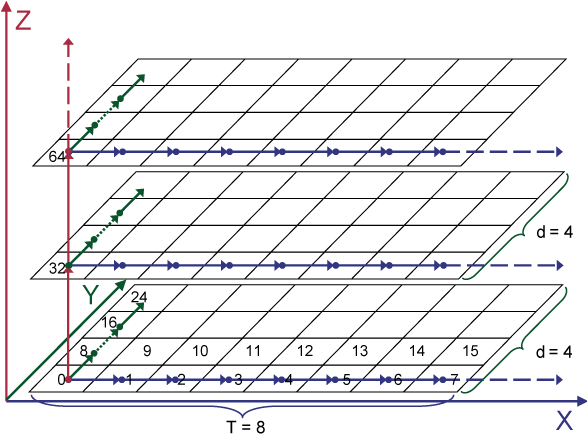
Figure 12: Example of mapping a 3D dataset using
MultiMap. Each row in the graph represents a disk track with a length of 8
and each cell corresponds to a disk block whose lbn is the
number inside the box. Suppose the value of d is 4.
Dimension X is mapped to the sequential blocks on the same
track. Dimension Y is mapped to the sequence of the first
adjacent blocks. For example, lbn 8 is the first adjacent
block of lbn 0 and lbn 16 is the first adjacent block of
lbn 8, etc. Dimension Z is mapped to the sequence of the 4th
adjacent blocks. For instance, lbn 32 is the 4th adjacent
block of lbn 0 and lbn 64 is the 4th adjacent of lbn
32. In this way, MultiMap utilizes the adjacent blocks with
different steps to preserve locality on the disk.
MultiMap preserves the spatial locality in the sense that
neighboring points in the geometric space will be stored in disk
blocks that are adjacent to each other, allowing for access with
minimal positioning cost. Since accessing the first adjacent
block and the d-th adjacent block has the same cost, we can
access up to d separate points that are equidistant from a
starting point. This mapping preserves the spatial relationship
that the next point along Y and the next point along
Z are equidistant (in terms of positioning cost) to the
same starting point. Retrieval along the X dimension
result in efficient sequential access; retrieval along Y or
Z result in semi-sequential accesses which are much more
efficient than random or even nearby access, as shown in Figure 9.
Note that MultiMap is not a simple mapping of the 3D data
set to the <cylinder,head,sector> tuple representing the
coordinates of the physical blocks on disk. MultiMap
provides a general approach for mapping N-dimensional data
sets to adjacent blocks. For a given disk, the maximum number of
dimensions that can be mapped efficiently is limited by d for that
disk, such that N ≤ log2(d)
+ 2. As the focus of this work is the analysis of the
principles behind multidimensional access and not the general data
layout algorithm, we provide the generalized algorithm, its
derivation, and the analysis of its limits elsewhere [31].
Our experimental setup uses the same hardware configuration as in
Section 4. Our prototype system consists of two
software components running on the same host machine: a logical volume
manager (LVM) and a database storage manager. In a production system,
the LVM would likely reside inside a storage array system separate
from the host machine. The prototype LVM implements the
GETADJACENT algorithm and exports a single logical volume
mapped across multiple disks. The database storage manager maps
multidimensional datasets by utilizing the GETADJACENT and
GETTRACKBOUNDARIES functions provided by the LVM. Based on the
query type, it issues appropriate I/Os to the LVM, which then breaks
these I/Os into proper requests to individual disks. Even when such
requests are issued out of order, the disk firmware scheduler will
reorder them to minimize the total positioning cost.
The datasets used for our experiments are stored on multiple disks
in our LVM. Akin to commercial disk arrays, the LVM uses disks of
the same type and utilizes only a part (slice) of the disk's total
space [9]. The slices in our experiments
are slightly less than half of the total disk capacity and span
one or more zones.
Even though our LVM generates requests to all the disks during our
experiments, we report performance results for only a single disk.
The reason is that we examine average I/O response times, which depend
only on the characteristics of a single disk drive. Using multiple
drives improves the overall throughput, but does not affect the
relative performance comparisons of the three mappings that our
database storage manager implements: Naive, Hilbert, and
MultiMap.
We evaluate two types of spatial queries. Beam queries are
one-dimensional queries retrieving data points along lines parallel to
the cardinal dimensions of the dataset. Range queries, called
p-length cube queries, fetch a cube with an edge length equal to
the p% of the dataset's edge length.
The 3D dataset used in this experiment contains
1024×1024×1024 cells, where each cell maps to a distinct
LBN of the logical volume and contains as many data points as can
fit. We partition the space into chunks that each fit on a portion of
a single disk. For both disks, MultiMap uses d=128 and
conservatism of 30°.
|
|
| (a) Beam queries |
|
|
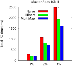
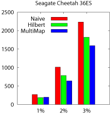
| (b) Range queries |
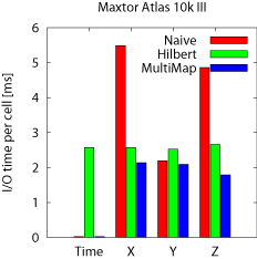
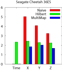
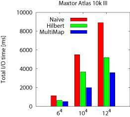
Figure 13: Performance using the 3D dataset.
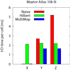
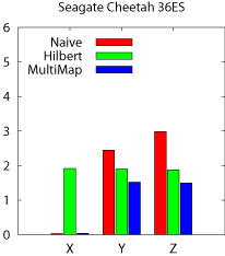
Beam queries The results for beam queries are presented in
Figure 13a. We run beam queries along all three
dimensions, X, Y, and Z, and the graphs show the average I/O
time per cell (disk block). As expected, the MultiMap model delivers
the best performance for all dimensions. It matches the streaming
performance of Naive along X. More importantly, MultiMap
outperforms Hilbert for Y and Z by 25%---35% and Naive by
62%--214% for the two disks. Finally, MultiMap achieves almost
identical performance on both disks unlike Hilbert and
Naive. That is because these disks have comparable settle times,
which affect the performance of accessing adjacent blocks for Y
and Z.
Range queries The first set of three bars, labeled 1% in
Figure 13b, shows the performance of 1%-length cube
queries expressed as their total runtime. As before, the performance
of each scheme follows the trends observed for the beam queries.
MultiMap improves the query performance (averaged across the two disks
and the three query types) by 37% and 11% respectively compared to
Naive and Hilbert. Both MultiMap and Hilbert outperform
Naive as it cannot employ sequential access for range
queries. MultiMap outperforms Hilbert, as Hilbert must fetch
some cells from physically distant disk blocks, although they are
close in the original dataset. These jumps make Hilbert less
efficient compared to MultiMap's semi-sequential accesses.
To examine the sensitivity of the cube query size, we also run
2%-length and 3%-length cube queries, whose results are presented in
the second and third sets of bars in Figure 13b. The
trends are similar, with MultiMap outperforming Hilbert and
Naive. The total run time increases because each query fetches more
data.
|
|
| (a) Beam queries |
|
|
| (b) Range queries |
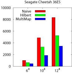
Figure 14: Performance using the 4D dataset.
In earthquake simulation, we use a 3D grid to model the 3D region of
the earth. The simulation computes the motion of the ground at each
node in the grid, for a number of discrete time steps. The 4D
simulation output contains a set of 3D grids, one for each step.
Our dataset is a 2000×64×64×64 grid modeling a
14 km deep slice of earth of a 38×38 km area in the
vicinity of Los Angeles with a total size of 250 GB of
data. 2000 is the total number of time steps. We choose time as the
primary dimension for the Naive and the MultiMap schemes and
partition the space into chunks that fit in a single disk.
The results, presented in Figure 14, exhibit the
same trends as the 3D experiments. The MultiMap model again achieves
the best performance for all beam and range queries. In
Figure 14a, the unusually good performance of Naive
on Y is due to a particularly fortunate mapping that results in
strided accesses that do not incur any rotational latency. The ratio
of strides to track sizes also explains the counterintuitive trend of
the Naive scheme's performance on the Cheetah disk where Z
outperforms Y, and Y outperforms X. The range queries, shown in
Figure 14b, perform on both disks as expected from the
3D case. In summary, MultiMap is efficient for processing queries
against spatio-temporal datasets, such as this earthquake simulation
output, and is the only scheme that can combine streaming performance
for time-varying accesses with efficient spatial access, thanks to the
preservation of locality on disk.
The work presented here exploits disk drive technology trends. It
improves access to multidimensional datasets by allowing the spatial
locality of the data to be preserved in the disk itself. Through
analysis of the characteristics of several state-of-the-art disk
drives, we show how to efficiently access non-contiguous adjacent
LBNs, which are hundreds of tracks away. Such accesses can be
readily realized with the existing disk firmware functions and
mappings of LBNs to physical locations.
Using our prototype implementation built with real, off-the-shelf disk
drives, we demonstrate that applications can utilize streaming
bandwidth for accesses along one dimension and efficient semi-sequential
accesses in the other N-1 dimensions. To the best of our knowledge,
this is the first approach that can preserve spatial locality of
stored multidimensional data, thus improving performance over current
data placement techniques.
We thank John Bucy for his years of effort developing and maintaining
the disk models that we use for this work. We thank the members and
companies of the PDL Consortium (including APC, EMC, EqualLogic,
Hewlett-Packard, Hitachi, IBM, Intel, Microsoft, Network Appliance,
Oracle, Panasas, Seagate, and Sun) for their interest, insights,
feedback, and support. We also thank IBM, Intel, and Seagate for
hardware donations that enabled this work. This work is funded in
part by NSF grants IIS-0133686 and CCR-0205544, by a Microsoft
Research Grant, and by an IBM faculty partnership award.
[1] L. Richard Carley, James A. Bain, Gary
K. Fedder, David W. Greve, David F. Guillou, Michael S. C. Lu,
Tamal Mukherjee, Suresh Santhanam, Leon Abelmann, and Seungook
Min. Single-chip computers with microelectromechanical
systems-based magnetic memory. Journal of Applied Physics,
87(9):6680-6685, 1 May 2000.
[1] K. A. S. Abdel-Ghaffar and
A. E. Abbadi. Optimal Allocation of Two-Dimensional
Data. International Conference on Database Theory (Delphi, Greece),
pages 409-418, January 8-10, 1997.
[2] V. Akcelik, J. Bielak, G. Biros,
I. Epanomeritakis, A. Fernandez, O. Ghattas, E. J. Kim, J. Lopez,
D. O�Hallaron, T. Tu, and J. Urbanic. High Resolution Forward And
Inverse Earthquake Modeling on Terascale Computers. ACM/IEEE
Conference on Supercomputing, page 52, 2003.
[3] D. Anderson, J. Dykes, and E. Riedel. More
than an interface: SCSI vs. ATA. Conference on File and Storage
Technologies (San Francisco, CA, 31 March-02 April 2003), pages
245-257. USENIX Association, 2003.
[4] M. J. Atallah and S. Prabhakar. (Almost)
Optimal Parallel Block Access for Range Queries. ACM
SIGMOD-SIGACT-SIGART Symposium on Principles of Database Systems
(Dallas, Texas, USA), pages 205-215. ACM, 2000.
[5] R. Bhatia, R. K. Sinha, and
C.-M. Chen. Declustering Using Golden Ratio Sequences. ICDE, pages
271-280, 2000.
[6] P. M. Chen and D. A. Patterson. Maximizing
performance in a striped disk array. UCB/CSD 90/559. Computer
Science Div., Department of Electrical Engineering and Computer
Science, University of California at Berkeley, February 1990.
[7] P. M. Deshpande, K. Ramasamy, A. Shukla, and
J. F. Naughton. Caching multidimensional queries using chunks. ACM
SIGMOD International Conference on Management of Data, pages
259-270. ACM Press, 1998.
[8] The DiskSim Simulation Environment (Version
3.0). http://www.pdl.cmu.edu/DiskSim/index.html.
[9] EMC Corporation. EMC Symmetrix DX3000 Product
Guide, http://www.emc.com/products/systems/DMX series.jsp, 2003.
[10] C. Faloutsos. Multiattribute hashing using
Gray codes. ACM SIGMOD, pages 227-238, 1986.
[11] C. Faloutsos and P. Bhagwat. Declustering
Using Fractals. International Conference on Parallel and
Distributed Information Systems (San Diego, CA, USA), 1993.
[12] V. Gaede and O. G�unther. Multidimensional
Access Methods. ACM Comput. Surv., 30(2):170-231, 1998.
[13] G. G. Gorbatenko and
D. J. Lilja. Performance of twodimensional data models for I/O
limited non-numeric applications. Laboratory for Advanced Research
in Computing Technology and Compilers Technical report
ARCTiC--02--04. University of Minnesota, February 2002.
[14] J. Gray, A. Bosworth, A. Layman, and
H. Pirahesh. Data Cube: A Relational Aggregation Operator
Generalizing Group-By, Cross-Tab, and Sub-Total. ICDE, pages
152-159. IEEE Computer Society, 1996.
[15] J. Gray, D. Slutz, A. Szalay, A. Thakar,
J. vandenBerg, P. Kunszt, and C. Stoughton. Data Mining the SDSS
Skyserver Database. Technical report. Microsoft Research, 2002.
[16] A. Guttman. R-Trees: A Dynamic Index
Structure for Spatial Searching. ACM SIGMOD, pages 47-57, 1984.
[17] D. Hilbert. U� ber die stetige Abbildung
einer Linie auf Fl�achenst�uck. Math. Ann, 38:459-460, 1891.
[18] H. V. Jagadish, L. V. S. Lakshmanan, and
D. Srivastava. Snakes and sandwiches: optimal clustering strategies
for a data warehouse. SIGMOD Rec., 28(2):37-48. ACM Press, 1999.
[19] N. Koudas, C. Faloutsos, and
I. Kamel. Declustering Spatial Databases on a Multi-Computer
Architecture. International Conference on Extending Database
Technology (Avignon, France), 1996.
[20] B. Moon, H. V. Jagadish, C. Faloutsos, and
J. H. Saltz. Analysis of the clustering properties of Hilbert
space-filling curve. Technical report. University of Maryland at
College Park, 1996.
[21] Office of Science Data-Management
Workshops. The Office of Science Data-Management
Challenge. Technical report. Department of Energy, 2005.
[22] J. A. Orenstein. Spatial query processing in
an object-oriented database system. ACM SIGMOD, pages
326-336. ACM Press, 1986.
[23] S. Prabhakar, K. Abdel-Ghaffar, D. Agrawal,
and A. E. Abbadi. Efficient Retrieval of Multidimensional Datasets
through Parallel I/O. International Conference on High Performance
Computing, page 375. IEEE Computer Society, 1998.
[24] C. Ruemmler and J. Wilkes. An introduction
to disk drive modeling. IEEE Computer, 27(3):17-28, March 1994.
[25] J. Schindler and G. R. Ganger. Automated
disk drive characterization. Technical report
CMU--CS--99--176. Carnegie-Mellon University, Pittsburgh, PA,
December 1999.
[26] J. Schindler, J. L. Griffin, C. R. Lumb, and
G. R. Ganger. Track-aligned extents: matching access patterns to
disk drive characteristics. Conference on File and Storage
Technologies (Monterey, CA, 28-30 January 2002), pages
259-274. USENIX Association, 2002.
[27] J. Schindler, S. W. Schlosser, M. Shao,
A. Ailamaki, and G. R. Ganger. Atropos: a disk array volume
manager for orchestrated use of disks. Conference on File and
Storage Technologies (San Francisco, CA, 31 March-02 April
2004). USENIX Association, 2004.
[28] S. W. Schlosser, J. Schindler, A. Ailamaki,
and G. R. Ganger. Exposing and exploiting internal parallelism in
MEMS-based storage. Technical Report
CMU--CS--03--125. Carnegie-Mellon University, Pittsburgh, PA, March
2003.
[29] M. Seltzer, P. Chen, and J. Ousterhout. Disk
scheduling revisited. Winter USENIX Technical Conference
(Washington, DC, 22-26 January 1990), pages 313-323, 1990.
[30] M. Shao, J. Schindler, S. W. Schlosser,
A. Ailamaki, and G. R. Ganger. Clotho: Decoupling memory page
layout from storage organization. International Conference on Very
Large Databases (Toronto, Canada, 31 August-2 September 2004),
2004.
[31] M. Shao, S. W. Schlosser,
S. Papadomanolakis, J. Schindler, A. Ailamaki, C. Faloutsos, and
G. R. Ganger. MultiMap: Preserving disk locality for
multidimensional datasets. Carnegie Mellon University Parallel Data
Lab Technical Report CMU--PDL--05--102. March 2005.
[32] A. Shukla, P. Deshpande, J. F. Naughton, and
K. Ramasamy. Storage Estimation for Multidimensional Aggregates in
the Presence of Hierarchies. International Conference on Very Large
Databases, pages 522-531. Morgan Kaufmann Publishers Inc., 1996.
[33] K. Stockinger, D. Dullmann, W. Hoschek, and
E. Schikuta. Improving the Performance of High-Energy Physics
Analysis through Bitmap Indices. Database and Expert Systems
Applications, pages 835-845, 2000.
[34] T. Stoehr, H. Maertens, and
E. Rahm. Multi-Dimensional Database Allocation for Parallel Data
Warehouses. International Conference on Very Large Databases, pages
273-284. Morgan Kaufmann Publishers Inc., 2000.
[35] N. Talagala, R. H. Arpaci-Dusseau, and
D. Patterson. Microbenchmark-based extraction of local and global
disk characteristics. Technical report
CSD--99--1063. University of California at Berkeley, 13 June
2000.
[36] B. L. Worthington, G. R. Ganger, and
Y. N. Patt. Scheduling algorithms for modern disk drives. ACM
SIGMETRICS Conference on Measurement and Modeling of Computer
Systems (Nashville, TN, 16-20 May 1994), pages 241-251. ACM
Press, 1994.
[37] B. L. Worthington, G. R. Ganger, Y. N. Patt,
and J. Wilkes. Online extraction of SCSI disk drive parameters. ACM
SIGMETRICS Conference on Measurement and Modeling of Computer
Systems (Ottawa, Canada), pages 146-156, May 1995.
[38] H. Yu, D. Agrawal, and A. E. Abbadi. Tabular
placement of relational data on MEMS-based storage
devices. International Conference on Very Large Databases (Berlin,
Germany, 09-12 September 2003), pages 680-693, 2003.
[39] H. Yu, K.-L. Ma, and J. Welling. Automated
Design of Multidimensional Clustering Tables for Relational
Databases. International Conference on Very Large Databases, 2004.
[40] H. Yu, K.-L. Ma, and J. Welling. A Parallel
Visualization Pipeline for Terascale Earthquake
Simulations. ACM/IEEE conference on Supercomputing, page 49, 2004.
[41] Y. Zhao, P. M. Deshpande, and
J. F. Naughton. An array-based algorithm for simultaneous
multidimensional aggregates. ACM SIGMOD International Conference on
Management of Data (Tucson, AZ, 13-15 May 1997). Published as
SIGMOD Record, 26(2):159-170. ACM, 1997.
|