 Subsections
![\includegraphics[angle=0,width=8.5cm]{graphics/visio/PacketPair}](img2.png)
|
The packet pair property of FIFO-queueing networks predicts the difference in arrival times of two packets of the same size traveling from the same source to the same destination:
The intuitive rationale for this equation (a full proof is given in
[LB00]) is that if two packets are sent close enough together
in time to cause the packets to queue together at the bottleneck link
(
![]() > t10 - t00), then the packets will
arrive at the destination with the same spacing (
t1n - t0n) as
when they exited the bottleneck link (
> t10 - t00), then the packets will
arrive at the destination with the same spacing (
t1n - t0n) as
when they exited the bottleneck link (
![]() ). The
spacing will remain the same because the packets are the same size and
no link downstream of the bottleneck link has a lower bandwidth than
the bottleneck link (as shown in Figure 1, which is
a variation of a figure from [Jac88]).
). The
spacing will remain the same because the packets are the same size and
no link downstream of the bottleneck link has a lower bandwidth than
the bottleneck link (as shown in Figure 1, which is
a variation of a figure from [Jac88]).
This property makes several assumptions that may not hold in practice. First, it assumes that the two packets queue together at the bottleneck link and at no later link. This could by violated by other packets queueing between the two packets at the bottleneck link, or packets queueing in front of the first, the second or both packets downstream of the bottleneck link. If any of these events occur, then Equation 1 does not hold. In Section 2.2, we describe how to mitigate this limitation by filtering out samples that suffer undesirable queueing.
In addition, the packet pair property assumes that the two packets are sent close enough in time that they queue together at the bottleneck link. This is a problem for very high bandwidth bottleneck links and/or for passive measurement. For example, from Equation 1, to cause queueing between two 1500 byte packets at a 1Gb/s bottleneck link, they would have to be transmitted no more than 12 microseconds apart. An active technique is more likely than a passive one to satisfy this assumption because it can control the size and transmission times of its packets. However, in Section 2.2, we describe how passive techniques can detect this problem and sometimes filter out its effect.
Another assumption of the packet pair property is that the bottleneck router uses FIFO-queueing. If the router uses fair queueing, then packet pair measures the available bandwidth of the bottleneck link [Kes91].
Finally, the packet pair property assumes that transmission delay is proportional to packet size and that routers are store-and-forward. The assumption that transmission delay is proportional to packet size may not be true if, for example, a router manages its buffers in such a way that a 128 byte packet is copied more than proportionally faster than a 129 byte packet. However, this effect is usually small enough to be ignored. The assumption that routers are store-and-forward (they receive the last bit of the packet before forwarding the first bit) is almost always true in the Internet.
Using the packet pair property, we can solve Equation 1 for bl, the bandwidth of the bottleneck link:
In this section, we describe in more detail how the assumptions in Section 2.1 can be violated in practice and how we can filter out this effect. Using measurements of the sizes and transmission and arrival times of several packets and Equation 1, we can get samples of the received bandwidth. The goal of a filtering technique is to determine which of these samples indicate the bottleneck link bandwidth and which do not. Our approach is to develop a filtering function that gives higher priority to the good samples and lower priority to the bad samples.
![\includegraphics[angle=0,width=12cm]{graphics/visio/PacketPairCases}](img9.png)
|
Before describing our filtering functions, we differentiate between the kinds of samples we want to keep and those we want to filter out. Figure 2 shows one case that satisfies the assumptions of the packet pair property and three cases that do not. There are other possible scenarios but they are combinations of these cases.
Case A shows the ideal packet pair case: the packets are sent sufficiently quickly to queue at the bottleneck link and there is no queueing after the bottleneck link. In this case the bottleneck bandwidth is equal to the received bandwidth and we do not need to do any filtering.
In case B, one or more packets queue between the first and second packets, causing the second packet to fall farther behind than would have been caused by the bottleneck link. In this case, the received bandwidth is less than the bottleneck bandwidth by some unknown amount, so we should filter this sample out.
In case C, one or more packets queue before the first packet after the bottleneck link, causing the second packet to follow the first packet closer than would have been caused by the bottleneck link. In this case, the received bandwidth is greater than the bottleneck bandwidth by some unknown amount, so we should filter this sample out.
In case D, the sender does not send the two packets close enough together, so they do not queue at the bottleneck link. In this case, the received bandwidth is less than the bottleneck bandwidth by some unknown amount, so we should filter this sample out. Active techniques can avoid case D samples by sending large packets with little spacing between them, but passive techniques are susceptible to them. Examples of case D traffic are TCP acknowledgements, voice over IP traffic, remote terminal protocols like telnet and ssh, and instant messaging protocols.
![\includegraphics[angle=0,width=9cm]{graphics/visio/FilteringKernelDensity}](img10.png)
|
To filter out the effect of case B and C, we use the insight that samples influenced by cross traffic will tend not to correlate with each other while the case A samples will correlate strongly with each other [Pax97] [CC96b]. This is because we assume that cross traffic will have random packet sizes and will arrive randomly at the links along the path. In addition, we use the insight that packets sent with a low bandwidth that arrive with a high bandwidth are definitely from case C and can be filtered out [Pax97]. Figure 3 shows a hypothetical example of how we apply these insights. Using the second insight, we eliminate the case C samples above the received bandwidth = sent bandwidth (x = y) line. Of the remaining samples, we calculate their smoothed distribution and pick the point with the highest density as the bandwidth.
There are many ways to compute the density function of a set of samples [Pax97] [CC96b], including using a histogram. However, histograms have the disadvantages of fixed bin widths, fixed bin alignment, and uniform weighting of points within a bin. Fixed bin widths make it difficult to choose an appropriate bin width without previously knowing something about the distribution. For example, if all the samples are around 100,000, it would not be meaningful to choose a bin width of 1,000,000. On the other hand, if all the samples are around 100,000,000, a bin width of 10,000 could flatten an interesting maxima. Another disadvantage is fixed bin alignment. For example, two points could lie very close to each other on either side of a bin boundary and the bin boundary ignores that relationship. Finally, uniform weighting of points within a bin means that points close together will have the same density as points that are at opposite ends of a bin. The advantage of a histogram is its speed in computing results, but we are more interested in accuracy and robustness than in saving CPU cycles.
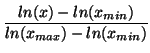
To avoid these problems, we use kernel density estimation [Sco92]. The idea is to define a kernel function K(t) with the property
![\includegraphics[angle=0,width=8.5cm]{graphics/visio/FilteringReceivedSentRatio}](img20.png)
|
Although density estimation is the best indicator in many situations, many case D samples can fool density estimation. For example, a host could transfer data in two directions over two different TCP connections to the same correspondent host. If data mainly flows in the forward direction, then the reverse direction would consist of many TCP acknowledgements sent with large spacings and a few data packets sent with small spacings. Figure 4 shows a possible graph of the resulting measurement samples. Density estimation would indicate a bandwidth lower than the correct one because there are so many case D samples resulting from the widely spaced acks.
We can improve the accuracy of our results if we favor samples that show evidence of actually causing queueing at the bottleneck link [LB99]. The case D samples are unlikely to have caused queueing at the bottleneck link because they are so close to the line x = y. On the other hand, the case A samples are on average far from the x = y line, meaning that they were sent with a high bandwidth but received with a lower bandwidth. This suggests that they did queue at the bottleneck link.
Using this insight we define the received/sent bandwidth ratio of a received bandwidth sample x to be
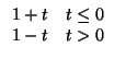
Unfortunately, given two samples with the same sent bandwidth (7) favors the one with the smaller received bandwith. To counteract this, we define the received bandwidth ratio to be
We can compose the filtering algorithms described in the previous sections by normalizing their values and taking their linear combination:
In addition to using a filtering function, we also only use the last w bandwidth samples. This allows us to quickly detect changes in bottleneck link bandwidth (agility) while being resistant to cross traffic (stability). A large w is more stable than a small w because it will include periods without cross traffic and different sources of cross traffic that are unlikely to correlate with a particular received bandwidth. However, a large w will be less agile than a small w for essentially the same reason. It is not clear to us how to define a w for all situations, so we currently punt on the problem by making it a user-defined parameter in nettimer.
Kevin Lai 2001-01-29

 + 0.3*p(x) + 0.3*r(x)